In this tutorial, we show how to turn an implementation of binary search into a
TLA+ specification. This implementation is known to have an out-of-bounds
error, which once existed in Java, see Nearly All Binary Searches and
Mergesorts are Broken by Joshua Bloch (2006). Our goal is to write a
specification after this implementation, not to write a specification of an
abstract binary search algorithm. You can find such a specification and a proof
in Proving Safety Properties and Binary search with a TLAPS proof by
Leslie Lamport (2019).
This tutorial is written under the assumption that the reader does not have any
knowledge of TLA+ and Apalache. Since we are not diving into protocol and
algorithm specifications too quickly, this is a nice example to start with. We
demonstrate how to use Apalache to find errors that are caused by integer
overflow and the out-of-bounds error, which is caused by this overflow. We
also show that the same overflow error prevents the algorithm from terminating
in the number of steps that is expected from the binary search. Normally it is
expected that the binary search terminates in log2(n) steps, where n is the
length of the search interval.
Sometimes, we refer to the model checker TLC in this text. TLC is another
model checker for TLA+ and was introduced in the late 90s. If you are new
to TLA+ and want to learn more about TLC, check the TLC project and the
TLA+ Video Course by Leslie Lamport. If you are an experienced TLC user,
you will find this tutorial helpful too, as it demonstrates the strong points
of Apalache.
We assume that you have Apalache installed. If not, check the manual page on
Apalache installation. The minimal required version is 0.22.0.
We provide all source files referenced in this tutorial as a ZIP archive
download. We still recommend that you follow along typing the TLA+ examples
yourself.
1:     public static int binarySearch(int[] a, int key) {
2:         int low = 0;
3:         int high = a.length - 1;
4:
5:         while (low <= high) {
6:             int mid = (low + high) / 2;
7:             int midVal = a[mid];
8:
9:             if (midVal < key)
10:                 low = mid + 1
11:             else if (midVal > key)
12:                 high = mid - 1;
13:             else
14:                 return mid; // key found
15:         }
16:         return -(low + 1);  // key not found.
17:     }
As was found by Joshua Bloch, the addition in line 6 may throw
an out-of-bounds exception at line 7, due to an integer overflow. This is because low
and high are signed integers, with a maximum value of 2^31 - 1.
However, the sum of two values, each smaller than 2^31-1, may be greater than 2^31 -1.
If this is the case, low + high can wrap into a negative number.
This bug was
discussed
in the TLA+ User Group in 2015. Let's see how TLA+ and Apalache can help us
here. A bit of warning: The final TLA+ specification will happen to be longer
than the 17 lines above. Don't get disappointed too fast. There are several
reasons for that:
TLA+ is not tuned towards one particular class of algorithms, e.g.,
sequential algorithms.
Related to the previous point, TLA+ and Apalache are not tuned to C or Java
programs. A software model checker such as CBMC, Stainless, or
Coral would probably accept a shorter program, and it would check it
faster. However, if you have a sledgehammer like TLA+, you don't have to learn
other languages.
We explicitly state the expected properties of the algorithm to be checked
by Apalache. In imperative languages, these properties are usually omitted or
written as plain-text comments.
We have to introduce a bit of boilerplate, to make Apalache work.
TLA+ is built around the concept of a state machine. The specified system
starts in a state that is picked from the set of its initial states. This
set of states is described with a predicate over states in TLA+. This predicate
is usually called Init. Further, the state machine makes a transition from
the current state to a successor state. These transitions are described with a
predicate over pairs of states (current, successor) in TLA+. This predicate
is usually called Next.
We start with the simplest possible specification of a single-state machine.
If we visualize it as a state diagram, it looks like follows:
Let's open a new file called BinSearch0.tla and type a very minimal module
definition:
This module does not yet specify any part of the binary search implementation.
However, it contains a few important things:
It imports constants and operators from three standard modules: Integers,
Sequences, and Apalache.
It declares the predicate Init. This predicate describes the initial
states of our state machine. Since we have not declared any variables, it
defines the single possible state.
It declares the predicate Next. This predicate describes the transitions
of our state machine. Again, there are no variables and Next == TRUE, so
this transition defines the entire set of states as reachable in a single
step.
Now it is a good time to check that Apalache works. Run the following command:
$ apalache-mc check BinSearch0.tla
The tool output is a bit verbose. Below, you can see the important lines of the
output:
...
PASS #13: BoundedChecker
Step 0: picking a transition out of 1 transition(s)
Step 1: picking a transition out of 1 transition(s)
...
Step 10: picking a transition out of 1 transition(s)
The outcome is: NoError
Checker reports no error up to computation length 10
...
We can see that Apalache runs without finding an error, as expected.
If you are curious, replace TRUE with FALSE in either Init or Next,
run Apalache again and observe what happens.
It is usually a good idea to start with a spec like BinSearch0.tla, to ensure
that the tools are working.
The Java code of binarySearch accepts two parameters: an array of integers
called a, and an integer called key. Similar to these parameters, we introduce
two specification parameters (called CONSTANTS in TLA+):
the input sequence INPUT_SEQ, and
the element to search for INPUT_KEY.
--------------------------- MODULE BinSearch1 ---------------------------------
EXTENDS Integers, Sequences, Apalache

CONSTANTS
    \* The input sequence.
    \*
    \* @type: Seq(Int);
    INPUT_SEQ,
    \* The key to search for.
    \*
    \* @type: Int;
    INPUT_KEY,
Importantly, the constants INPUT_SEQ and INPUT_KEY are prefixed with type
annotations in the comments:
INPUT_SEQ has the type Seq(Int), that is, it is a sequence of integers (sequences in TLA+ are indexed), and
INPUT_KEY has the type Int, that is, it is an integer.
Recall that we wanted to specify signed and unsigned Java integers, which are
32 bits long. TLA+ is not tuned towards any computer architecture. Its integers
are mathematical integers: always signed and arbitrarily large (unbounded).
To model fixed bit-width integers, we introduce another constant INT_WIDTH of
type Int:
    \* Bit-width of machine integers.
    \*
    \* @type: Int;
    INT_WIDTH
The benefit of defining the bit width as a parameter is that we can try
our specification for various bit widths of integers: 4-bit, 8-bit, 16-bit, 32-bit,
etc. Similar to many programming languages, we introduce several constant
definitions (a^b is a taken to the power of b):
\* the largest value of an unsigned integer
MAX_UINT == 2^INT_WIDTH
\* the largest value of a signed integer
MAX_INT  == 2^(INT_WIDTH - 1) - 1
\* the smallest value of a signed integer
MIN_INT  == -2^(INT_WIDTH - 1)
Note that these definitions do not constrain integers in any way. They are
simply convenient names for the constants that we will need in the
specification.
To make sure that the new specification does not contain syntax errors or
type errors, execute:
We start with the simplest possible case that occurs in binarySearch. Namely,
we consider the case where low > high, that is, binarySearch never enters
the loop.
Introduce variables. To do that, we have to finally introduce some
variables. Obviously, we have to introduce variables low and high. This is
how we do it:
VARIABLES
    \* The low end of the search interval (inclusive).
    \* @type: Int;
    low,
    \* The high end of the search interval (inclusive).
    \* @type: Int;
    high,
The variables low and high are called state variables. They define a state of our state machine.
That is, they are never introduced and never removed.
Remember, TLA+ is not tuned towards any particular computer
architecture, and thus it does not even have the notion of an execution stack.
You can think of low and high as being global variables. Yes, global
variables are generally frowned upon in programming languages. However, when dealing with a
specification, they are much easier to reason about than the execution stack.
We will demonstrate how to introduce local definitions later in this tutorial.
We introduce two additional variables, the purpose of which might be less obvious:
    \* Did the algorithm terminate.
    \* @type: Bool;
    isTerminated,
    \* The result when terminated.
    \* @type: Int;
    returnValue
The variable isTerminated indicates whether our search has terminated. Why do
we even have to introduce it? Because, some computer systems are not designed
with termination in mind. For instance, such distributed systems as the
Internet and Bitcoin are designed to periodically serve incoming requests
instead of producing a single output for a single input.
If we want to specify the Internet or Bitcoin, do we
understand what it means for them to terminate?
The variable returnValue will contain the result of the binary search, when
the search terminates. Recall, there is no execution stack. Hence, we introduce
the variable returnValue right away. The downside is that we have to do
bookkeeping for this variable.
Initialize variables. Having introduced the variables, we have to
initialize them. That is, we want to specify lines 2–3 of the Java code:
1:     public static int binarySearch(int[] a, int key) {
2:         int low = 0;
3:         int high = a.length - 1;
           ...
17:    }
To this end, we change the body of the predicate Init to the following:
You probably have guessed, what the above line means. Maybe you are a bit
puzzled about the mountain-like operator /\. It is called conjunction,
which is usually written as && or and in programming languages. The
important effect of the above expression is that every variable in the
left-hand side of = is required to have the value specified in the right-hand
side of =1.
As it is hard to fit many expressions in one line, TLA+ offers special syntax
for writing a big conjunction. Here is the standard way of writing Init
(indentation is important):
The above lines do not deserve a lot of explanation. As you have probably guessed,
Len(INPUT_SEQ) computes the length of the input sequence.
1
It is important to know that TLA+ does not impose any
particular order of evaluation for /\. However, both Apalache and TLC
evaluate some expressions of the form x = e in the initialization predicate
as assignments. Hence, it is often a good idea to think about /\ as being
evaluated from left to right.
Update variables. Having done all the preparatory work, we are now ready to
specify the behavior in lines 5 and 16 of binarySearch.
1:     public static int binarySearch(int[] a, int key) {
2:         int low = 0;
3:         int high = a.length - 1;
4:
5:         while (low <= high) {
            ...
15:        }
16:        return -(low + 1);  // key not found.
17:    }
To this end, we redefine Next as follows:
\* Computation step (lines 5-16)
Next ==
    IF ~isTerminated
    THEN IF low <= high
      THEN          \* lines 6-14: not implemented yet
        UNCHANGED <<low, high, isTerminated, returnValue>>
      ELSE          \* line 16
        /\ isTerminated' = TRUE
        /\ returnValue' = -(low + 1)
        /\ UNCHANGED <<low, high>>
Most likely, you have no problem reading this definition, except for the part
that includes isTerminated', returnValue', and UNCHANGED. Recall that a
transition predicate, like Next, specifies the relation between two states of
the state machine; the current state, the variables of which are referenced by
unprimed names, and the successor-state, the variables of which are referenced
by primed names.
The expression isTerminated' = TRUE means that only states where
isTerminated equals TRUE can be successors of the current state. In
general, isTerminated' could also depend on the value of isTerminated, but
here, it does not. Likewise, returnValue' = -(low + 1) means that
returnValue has the value -(low + 1) in the next state. The expression
UNCHANGED <<low, high>> is a convenient shortcut for writing low' = low /\ high' = high. Readers unfamiliar with specification languages might question
the purpose of UNCHANGED, since in most programming languages variables only
change when they are explicitly changed. However, a transition predicate, like
Next, establishes a relation between pairs of states. If we were to omit
UNCHANGED, this would mean that we consider states in which low and high
have completely arbitrary values as valid successors. This is clearly not
how Java code should behave. To encode Java semantics, we must therefore
explicitly state that low and high do not change in this step.
It is important to understand that an expression like returnValue' = -(low + 1)does not immediately update the variable on the left-hand side. Hence,
returnValue still refers to the value in the state before evaluation of
Next, whereas returnValue' refers to the value in the state that is
computed after evaluation of Next. You can think of the effect of x' = e
being delayed until the whole predicate Next is evaluated.
As we discussed, it is a good habit to periodically run the model checker, as you are writing
the specification. Even if it doesn't check much, you would be able to catch
the moment when the model checker slows down. This may give you a useful
hint about changing a few things before you have written too much code.
Let us check BinSearch2.tla:
$ apalache-mc check BinSearch2.tla
If it is your first TLA+ specification, you may be surprised by this error:
...
PASS #13: BoundedChecker
This error may show up when CONSTANTS are not initialized.
Check the manual: https://apalache.informal.systems/docs/apalache/parameters.html
Input error (see the manual): SubstRule: Variable INPUT_SEQ is not assigned a value
...
Apalache complains that we have declared several constants (INPUT_SEQ,
INPUT_KEY, and INT_WIDTH), but we have never defined them.
Adding a model file. The standard approach in this case is either to fix
all constants, or to introduce another module that
fixes the parameters and instantiates the general specification. Although
Apalache supports TLC Configuration Files, for the purpose of this tutorial,
we will stick to tool-agnostic TLA+ syntax.
To this end, we add a new file MC2_8.tla with the following contents:
-------------------------- MODULE MC2_8 ---------------------------------------
\* an instance of BinSearch2 with all parameters fixed

\* fix 8 bits
INT_WIDTH == 8
\* the input sequence to try
\* @type: Seq(Int);
INPUT_SEQ == << >>
\* the element to search for
INPUT_KEY == 10

\* introduce the variables to be used in BinSearch2
VARIABLES
    \* @type: Int;
    low,
    \* @type: Int;
    high,
    \* @type: Bool;
    isTerminated,
    \* @type: Int;
    returnValue

\* use an instance for the fixed constants
INSTANCE BinSearch2
===============================================================================
As you can see, we fix the values of all parameters. We are instantiating
the module BinSearch2 with these fixed parameters. Since instantiation
requires all constants and variables to be defined, we copy the variables
definitions from BinSearch2.tla.
Since we are fixing the parameters with concrete values, MC2_8.tla looks very
much like a unit test. It's a good start for debugging a few things, but since
our program is entirely sequential, our specification is as good as a unit
test. Later in this tutorial, we will show how to leverage Apalache to check
properties for all possible inputs (up to some bound).
Let us check MC2_8.tla:
$ apalache-mc check MC2_8.tla
...
Checker reports no error up to computation length 10
This time Apalache has not complained. This is a good time to stop and think
about whether the model checker has told us anything interesting. Kind of. It
told us that it has not found any contradictions. But it did not tell us
anything interesting about our expectations. Because we have not set our
expectations yet!
What do we expect from binary search? We can check the Java documentation,
e.g., Arrays.java in OpenJDK:
...the return value will be >= 0 if and only if the key is found.
This property is actually quite easy to write in TLA+. First, we
introduce the property that we call ReturnValueIsCorrect:
\* The property of particular interest is this one:
\*
\* "Note that this guarantees that the return value will be >= 0 if
\*  and only if the key is found."
ReturnValueIsCorrect ==
    LET MatchingIndices ==
        { i \in DOMAIN INPUT_SEQ: INPUT_SEQ[i] = INPUT_KEY }
    IN
    IF MatchingIndices /= {}
    THEN \* Indices in TLA+ start with 1, whereas the Java returnValue starts with 0
        returnValue + 1 \in MatchingIndices
    ELSE returnValue < 0
Let us decompose this property into smaller pieces. First, we define the set
MatchingIndices:
ReturnValueIsCorrect ==
    LET MatchingIndices ==
        { i \in DOMAIN INPUT_SEQ: INPUT_SEQ[i] = INPUT_KEY }
With this TLA+ expression we define a local constant called MatchingIndices
that is equal to the set of indices i in INPUT_SEQ so that the sequence
elements at these indices are equal to INPUT_KEY. If this syntax
is hard to parse for you, here is how we could write a similar definition in a
functional programming language (Scala):
val MatchingIndices =
    INPUT_SEQ.indices.toSet.filter { i => INPUT_SEQ(i) == INPUT_KEY }
Since the
sequence indices in TLA+ start with 1, we require that returnValue + 1
belongs to MatchingIndices when MatchingIndices is non-empty. If
MatchingIndices is empty, we require returnValue to be negative.
We can check that the property ReturnValueIsCorrect is an invariant, that
is, it holds in every state that is reachable from the states specified by Init
via a sequence of transitions specified by Next:
This property is violated in the initial state. To see why, check the file
counterexample1.tla.
Actually, we only expect this property to hold after the computation terminates,
that is, when isTerminated equals to TRUE. Hence, we add the following
invariant:
\* What we expect from the search when it is finished.
Postcondition ==
    isTerminated => ReturnValueIsCorrect
Digression: Boolean connectives. In the above code, the operator => is
the Classical implication. In general, A => B is equivalent to IF A THEN B ELSE TRUE. The implication A => B is also equivalent to the TLA+
expression ~A \/ B, which one can read as "not A holds, or B holds". The
operator \/ is called disjunction. As a reminder, here is the standard
truth table for the Boolean connectives, which are no different from the
Boolean logic in TLA+:
A
B
~A
A \/ B
A /\ B
A => B
FALSE
FALSE
TRUE
FALSE
FALSE
TRUE
FALSE
TRUE
TRUE
TRUE
FALSE
TRUE
TRUE
FALSE
FALSE
TRUE
FALSE
FALSE
TRUE
TRUE
FALSE
TRUE
TRUE
TRUE
Checking Postcondition.
Let us check Postcondition on MC3_8.tla:
$ apalache-mc check --inv=Postcondition MC3_8.tla
This property holds true. However, it's a small win, as MC3_8.tla fixes all
parameters. Hence, we have checked the property just for one data point. In
Step 5, we will check Postcondition for all sequences admitted by INT_WIDTH.
        LET mid == (low + high) \div 2 IN
        LET midVal == INPUT_SEQ[mid + 1] IN
As you have probably guessed, we define two (local) values mid and midVal.
The value mid is the average of low and high. The operator \div is
simply integer division, which is usually written as / or // in programming
languages. The value midVal is the value at the location mid + 1. Since
the TLA+ sequence INPUT_SEQ has indices in the range 1..Len(INPUT_SEQ),
whereas we are computing zero-based indices, we are adjusting the index by one,
that is, we write INPUT_SEQ[mid + 1] instead of INPUT_SEQ[mid].
Warning: The definitions of mid and midVal do not properly reflect the
Java code of binarySearch. We will fix them later. It is a good exercise
to stop here and think about the source of this imprecision.
The following lines look like ASCII graphics, but by now you should know
enough to read them:
These lines are the indented form of \/ for three cases:
when midVal < INPUT_KEY, or
when midVal > INPUT_KEY, or
when midVal = INPUT_KEY.
We could write these expressions with IF-THEN-ELSE or even with the TLA+
operator CASE (see Summary of TLA+). However, we find the disjunctive
form to be the least cluttered, though unusual.
Now we can check the postcondition again:
$ apalache-mc check --inv=Postcondition MC4_8.tla
The check goes through, but did it do much? Recall, that we fixed INPUT_SEQ
to be the empty sequence << >> in MC4_8.tla. Hence, we never enter the loop
we have just specified.
Actually, Apalache gives us a hint that it never tries some of the
cases:
...
PASS #13: BoundedChecker
State 0: Checking 1 state invariants
Step 0: picking a transition out of 1 transition(s)
Step 1: Transition #0 is disabled
Step 1: Transition #1 is disabled
Step 1: Transition #2 is disabled
Step 1: Transition #3 is disabled
State 1: Checking 1 state invariants
Step 1: picking a transition out of 1 transition(s)
Step 2: Transition #0 is disabled
Step 2: Transition #1 is disabled
Step 2: Transition #2 is disabled
Step 2: Transition #4 is disabled
Step 2: picking a transition out of 1 transition(s)
...
Digression: symbolic transitions. Internally, Apalache decomposes the
predicates Init and Next into independent pieces like Init == Init$0 \/ Init$1 and Next == Next$0 \/ Next$1 \/ Next$2 \/ Next$3. If you want to see
how it is done, run Apalache with the options --write-intermediate and --run-dir:
Check the file out/intermediate/XX_OutTransitionFinderPass.tla, which contains the
preprocessed specification that has Init and Next decomposed. You can find
a detailed explanation in the section on Assignments in Apalache.
In this step, we are going to check the invariant Postcondition for all
possible input sequences and all input keys (for a fixed bit-width).
Create the file MC5_8.tla with the following contents:
-------------------------- MODULE MC5_8 ---------------------------------------
\* an instance of BinSearch5 with all parameters fixed
EXTENDS Apalache

\* fix 8 bits
INT_WIDTH == 8

\* We do not fix INT_SEQ and INPUT_KEY.
\* Instead, we reason about all sequences with ConstInit.

CONSTANTS
    \* The input sequence.
    \*
    \* @type: Seq(Int);
    INPUT_SEQ,
    \* The key to search for.
    \*
    \* @type: Int;
    INPUT_KEY

\* introduce the variables to be used in BinSearch5
VARIABLES
    \* @type: Int;
    low,
    \* @type: Int;
    high,
    \* @type: Bool;
    isTerminated,
    \* @type: Int;
    returnValue

\* use an instance for the fixed constants
INSTANCE BinSearch5

==================
Note that we introduced INPUT_SEQ and INPUT_KEY as parameters again. We
cannot check MC5_8.tla just like that. If we try to check MC5_8.tla,
Apalache would complain again about a value missing for INPUT_SEQ.
ConstInit. This idiom allows us to initialize CONSTANTS with a TLA+
formula. Let us introduce the following operator definition in MC5_8.tla:
ConstInit ==
    /\ INPUT_KEY \in Int
    \* Seq(Int) is a set of all sequences that have integers as elements
    /\ INPUT_SEQ \in Seq(Int)
This is a straightforward definition. However, it does not work in Apalache:
$ apalache-mc check --cinit=ConstInit --inv=Postcondition MC5_8.tla
...
MC5_8.tla:39:22-39:29: unsupported expression: Seq(_) produces an infinite set of unbounded sequences.
Checker has found an error
...
The issue with our definition of ConstInit is that it requires the model
checker to reason about the infinite set of sequences, namely, Seq(Int).
Interestingly, the model checking does not complain about the expression
INPUT_KEY \in Int. The reason is that this expression requires the model
checker to reason about one integer, though it ranges over the infinite set of
integers.
Value generators. Fortunately, this problem can be easily circumvented by
using Apalache Value generators2.
In this new version, we use the Apalache operator Gen to:
produce an unrestricted integer to be used as a value of INPUT_KEY and
produce a sequence of integers to be used as a value of INPUT_SEQ. This
sequence is unrestricted, except its length is bounded with MAX_INT,
which is exactly what we need in our case study.
The operator Gen introduces a data structure of a proper type whose size is
bounded with the argument of Gen. For instance, the type of INPUT_SEQ is
the sequence of integers, and thus Gen(MAX_INT) produces an unrestricted
sequence of up to MAX_INT elements. This sequence is bound to the name
INPUT_SEQ. For details, see Value generators. This lets Apalache check
all instances of the data structure, without enumerating the instances!
By doing so, we are able to check the specification for all the inputs, when we
fix the bit width. To quickly get feedback from Apalache, we fix INT_WIDTH to 8 in the model MC5_8.tla.
2
If you know property-based testing, e.g., QuickCheck,
Apalache generators are inspired by this idea. In contrast to property-based
testing, an Apalache generator is not randomly producing values. Rather,
Apalache simply introduces an unconstrained data structure (e.g., a set, a
function, or a sequence) of the proper type. Hence, Apalache is reasoning about
all possible instances of this data structure, instead of reasoning about a
small set of randomly chosen instances.
Let us check Postcondition again:
$ apalache-mc check --cinit=ConstInit --inv=Postcondition MC5_8.tla
...
State 2: state invariant 0 violated. Check the counterexample in:
  /[a long path]/counterexample1.tla
...
If we check our source of truth, that is, the Java documentation in
Arrays.java in OpenJDK, we will see the following sentences:
The range must be sorted (as by the {@link #sort(int[], int, int)} method)
prior to making this call. If it is not sorted, the results are undefined.
If the range contains multiple elements with the specified value, there is
no guarantee which one will be found.
It is quite easy to add this constraint 3. This is where TLA+ starts to
shine:
InputIsSorted ==
    \* The most straightforward way to specify sortedness
    \* is to use two quantifiers,
    \* but that would produce O(Len(INPUT_SEQ)^2) constraints.
    \* Here, we write it a bit smarter.
    \A i \in DOMAIN INPUT_SEQ:
        i + 1 \in DOMAIN INPUT_SEQ =>
          INPUT_SEQ[i] <= INPUT_SEQ[i + 1]

...

\* What we expect from the search when it is finished.
PostconditionSorted ==
    isTerminated => (~InputIsSorted \/ ReturnValueIsCorrect)
If we check PostconditionSorted, we do not get any error after 10 steps:
$ apalache-mc check --cinit=ConstInit --inv=PostconditionSorted MC5_8.tla
...
The outcome is: NoError
Checker reports no error up to computation length 10
It takes some time to explore all executions of length up to 10 steps, for all
input sequences of length up to 2^7 - 1 arbitrary integers. If we think about
it, the model checker managed to crunch infinitely many numbers in several
hours. Not bad.
Exercise. If you are impatient, you can check PostconditionSorted for the
configuration that has integer width of 4 bits. It takes only a few seconds to
explore all executions.
3
Instead of checking whether INPUT_SEQ is sorted in the
post-condition, we could restrict the constant INPUT_SEQ to be sorted in
every execution. That would effectively move this constraint into the
pre-condition of the search. Had we done that, we would not be able to observe
the behavior of the search on the unsorted inputs. An important property is
whether the search is terminating on all inputs.
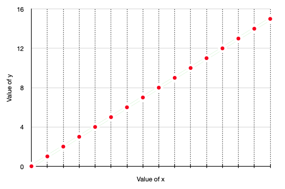
Actually, we do not need 10 steps to check termination for the case INT_WIDTH = 8. If you recall the complexity of the binary search, it needs
ceil(log2(Len(INPUT_SEQ))) steps to terminate.
To check this property, we add the number of steps as a variable in
BinSearch6.tla and in MC6_8.tla:
VARIABLES
    ...
    \* The number of executed steps.
    \* @type: Int;
    nSteps
Also, we update Init and Next in BinSearch6.tla as follows:
Init ==
    ...
    /\ nSteps = 0

Next ==
    IF ~isTerminated
    THEN IF low <= high
      THEN          \* lines 6-14
        /\ nSteps' = nSteps + 1
        /\ LET mid == (low + high) \div 2 IN
         ...
      ELSE          \* line 16
        /\ isTerminated' = TRUE
        /\ returnValue' = -(low + 1)
        /\ UNCHANGED <<low, high, nSteps>>
    ELSE            \* isTerminated
      UNCHANGED <<low, high, returnValue, isTerminated, nSteps>>
Having nSteps, we can write the Termination property:
\* We know the exact number of steps to show termination.
Termination ==
    (nSteps >= INT_WIDTH) => isTerminated
Let us check Termination:
$ apalache-mc check --cinit=ConstInit --inv=Termination MC6_8.tla
...
Checker reports no error up to computation length 10
It took me 0 days  0 hours  0 min 19 sec
Even if we did not know the precise complexity of the binary search, we could
write a simpler property, which demonstrates the progress of the search:
Do you recall that our specification of the loop had a caveat? Let us have a
look at this piece of the specification again:
    IF ~isTerminated
    THEN IF low <= high
      THEN          \* lines 6-14
        /\ nSteps' = nSteps + 1
        /\ LET mid == (low + high) \div 2 IN
           LET midVal == INPUT_SEQ[mid + 1] IN
            \//\ midVal < INPUT_KEY \* lines 9-10
              /\ low' = mid + 1
              /\ UNCHANGED <<high, returnValue, isTerminated>>
            \//\ midVal > INPUT_KEY \* lines 11-12
              /\ high' = mid -1
              /\ UNCHANGED <<low, returnValue, isTerminated>>
            \//\ midVal = INPUT_KEY \* lines 13-14
              /\ returnValue' = mid
              /\ isTerminated' = TRUE
              /\ UNCHANGED <<low, high>>
You can see that all arithmetic operations are performed over TLA+ integers,
that is, unbounded integers. We have to implement fixed-width integers ourselves.
Fortunately, we do not have to implement the whole set of integer operators,
but only the addition over signed integers, which has a potential to overflow.
To this end, we have to recall how signed integers are represented in modern
computers, see Two's complement. Fortunately, we do not have to worry about
an efficient implementation of integer addition. We simply use addition over
unbounded integers to implement addition over fixed-width integers:
\* Addition over fix-width integers.
IAdd(i, j) ==
    \* add two integers with unbounded arithmetic
    LET res == i + j IN
    IF MIN_INT <= res /\ res <= MAX_INT
    THEN res
    ELSE \* wrap the result over 2^INT_WIDTH (probably redundant)
        LET wrapped == res % MAX_UINT IN
        IF wrapped <= MAX_INT
        THEN wrapped    \* a positive integer, return as is
        ELSE \* complement the value to represent it with an unbounded integer
          -(MAX_UINT - wrapped)
Having defined IAdd, we replace addition over unbounded integers with IAdd:
Next ==
    IF ~isTerminated
    THEN IF low <= high
      THEN          \* lines 6-14
        /\ nSteps' = nSteps + 1
        /\ LET mid == IAdd(low, high) \div 2 IN
           LET midVal == INPUT_SEQ[mid + 1] IN
            \//\ midVal < INPUT_KEY \* lines 9-10
              /\ low' = IAdd(mid, 1)
              /\ UNCHANGED <<high, returnValue, isTerminated>>
            \//\ midVal > INPUT_KEY \* lines 11-12
              /\ high' = IAdd(mid, - 1)
              /\ UNCHANGED <<low, returnValue, isTerminated>>
            \//\ midVal = INPUT_KEY \* lines 13-14
              /\ returnValue' = mid
              /\ isTerminated' = TRUE
              /\ UNCHANGED <<low, high>>
      ELSE          \* line 16
        ...
This finally gives us a specification that faithfully represents the Java code
of binarySearch. Now we can check all expected properties once again:
$ apalache-mc check --cinit=ConstInit --inv=PostconditionSorted MC7_8.tla
...
State 2: state invariant 0 violated.
...
Total time: 2.786 sec
$ apalache-mc check --cinit=ConstInit --inv=Progress MC7_8.tla
...
State 1: action invariant 0 violated.
...
Total time: 2.935 sec
$ apalache-mc check --cinit=ConstInit --inv=Termination MC7_8.tla
...
State 8: state invariant 0 violated.
...
Total time: 39.540 sec
As we can see, all of our invariants are violated. They all demonstrate the
issue that is caused by the integer overflow!
As we have seen in Step 7, the cause of all errors in PostconditionSorted,
Termination, and Progress is that the addition low + high overflows and
thus the expression INPUT_SEQ[mid + 1] accesses INPUT_SEQ outside of its
domain.
Why did Apalache not complain about access outside of the domain? Its behavior
is actually consistent with Specifying Systems (p. 302):
A function f has a domain DOMAIN f, and the value of f[v] is
specified only if v is an element of DOMAIN f.
Hence, Apalache returns some value of a proper type, if v is outside of
DOMAIN f. As we have seen in Step 7, such a value would usually show up in a
counterexample. In the future, Apalache will probably have an automatic check
for out-of-domain access. For the moment, we can write such a check as a state
invariant. By propagating the conditions from INPUT_SEQ[mid + 1] up in Next,
we construct the following invariant:
\* Make sure that INPUT_SEQ is accessed within its bounds
InBounds ==
  LET mid == IAdd(low, high) \div 2 IN
  \* collect the conditions of IF-THEN-ELSE
  ~isTerminated =>
    ((low <= high) =>
      (mid + 1) \in DOMAIN INPUT_SEQ)
Apalache finds a violation of this invariant in a few seconds:
$ apalache-mc check --cinit=ConstInit --inv=InBounds MC8_8.tla
...
State 1: state invariant 0 violated.
...
Total time: 3.411 sec
If we check counterexample1.tla, it contains the following values for low
and high:
        /\ LET mid == IAdd(low, high) \div 2 IN
           LET midVal == INPUT_SEQ[mid + 1] IN
The fix is as follows:
        /\ LET mid == IAdd(low, IAdd(high, -low) \div 2) IN
           LET midVal == INPUT_SEQ[mid + 1] IN
We also update InBounds as follows:
\* Make sure that INPUT_SEQ is accessed within its bounds
InBounds ==
  LET mid == IAdd(low, IAdd(high, -low) \div 2) IN
...
Now we check the four invariants: InBounds, PostconditionSorted,
Termination, and Progress.
$ apalache-mc check --cinit=ConstInit --inv=InBounds MC9_8.tla
...
The outcome is: NoError
...
Total time: 76.352 sec
$ apalache-mc check --cinit=ConstInit --inv=Progress MC9_8.tla
...
The outcome is: NoError
...
Total time: 63.578 sec
$ apalache-mc check --cinit=ConstInit --inv=Termination MC9_8.tla
...
The outcome is: NoError
...
Total time: 72.682 sec
$ apalache-mc check --cinit=ConstInit --inv=PostconditionSorted MC9_8.tla
...
The outcome is: NoError
...
Total time: 2154.646 sec
Exercise: It takes quite a bit of time to check PostconditionSorted.
Change INT_WIDTH to 6 and check all these invariants once again. Observe that
it takes Apalache significantly less time.
Exercise: Change INT_WIDTH to 16 and check all these invariants once again.
Observe that it takes Apalache significantly more time.
We have reached our goals: TLA+ and Apalache helped us in finding the access
bug and showing that its fix works. Now it is time to look back at the
specification and make it easier to read.
The definitions LoopIteration, LoopExit, and StutterOnTermination are
called actions in TLA+. It is usually a good idea to decompose a large Next
formula into actions. Normally, an action contains assignments to all primed
variables.
Specify the behavior of a sequential algorithm (binary search).
Specify invariants that check safety and termination.
Take into account the specifics of a computer architecture (fixed bit
width).
Automatically find examples of simultaneous invariant violation.
Efficiently check the expected properties against our specification.
We have written our specification for parameterized bit width. This lets us
check the invariants relatively quickly and get fast feedback from the model
checker. We chose a bit width of 8, a non-trivial value for which
Apalache terminates within a reasonable time. Importantly, the specification
for the bit width of 32 stays the same; we only have to change INT_WIDTH. Of
course, Apalache reaches its limits when we set INT_WIDTH to 16 or 32. In
these cases, it has to reason about all sequences of length up to 32,767
elements or 2 Billion elements, respectively!
Apalache gives us a good idea whether the properties of our
binary search specification hold true. However, it does not give us an ultimate proof of correctness for
Java integers. If you need such a proof, you should probably use TLAPS. Check
the paper on Proving Safety Properties by Leslie Lamport.
This tutorial is rather long. This is because we wanted to show the evolution
of a TLA+ specification, as we were writing it and checking it with Apalache.
There are many different styles of writing TLA+ specifications. One of our
goals was to demonstrate the incremental approach to specification writing. In
fact, this approach is not very different from incremental development of
programs in the spirit of Test-driven development. It took us 2 to 3 hours to
iteratively develop a specification that is similar to the one demonstrated in
this tutorial.
This tutorial touches upon the basics of TLA+ and Apalache. For instance, we
did not discuss non-determinism, as our specification is entirely
deterministic. We will demonstrate advanced features in future tutorials.
If you are experiencing a problem with Apalache, feel free to open an issue
or drop us a message on Zulip chat.
In this tutorial, we introduce the Snowcat ❄ 🐱 type checker.
We give concrete steps to running the type checker and annotating a specification
with types.
This tutorial uses Type System 1.2, which guarantees safe record access. To see
how to upgrade to Type System 1.2, check Migrating to Type System 1.2.
As a running example, we are using the specification of Lamport's Mutex
(written by Stephan Merz). We recommend to reproduce the steps in this
tutorial. So, go ahead and download the specification file
LamportMutex.tla. We will add type annotations to this file. Let's rename
LamportMutex.tla to LamportMutexTyped.tla.
In Step 1, Snowcat complained about the name clock. The reason
for that is very simple: clock is declared as a variable, but Snowcat
does not find a type annotation for it.
The comment next to the declaration of clock does not tell us precisely
what clock should be:
clock, \* local clock of each process
Let's dig a bit further and check TypeOK, which is usually a good source of
type hints in untyped specifications:
TypeOK ==
     (* clock[p] is the local clock of process p *)
  /\ clock \in [Proc -> Clock]
     (* req[p][q] stores the clock associated with request from q received by p, 0 if none *)
  /\ req \in [Proc -> [Proc -> Nat]]
     (* ack[p] stores the processes that have ack'ed p's request *)
  /\ ack \in [Proc -> SUBSET Proc]
     (* network[p][q]: queue of messages from p to q -- pairwise FIFO communication *)
  /\ network \in [Proc -> [Proc -> Seq(Message)]]
     (* set of processes in critical section: should be empty or singleton *)
  /\ crit \in SUBSET Proc
This is better, but we have to figure out the types of Proc and Clock.
Let's have a look at their definitions.
Proc == 1 .. N
Clock == Nat \ {0}
From the definitions of Proc and Clock, it is clear that they are both
subsets of integers. We could annotate these two definitions with the type
Set(Int), but this is not necessary, since Snowcat will infer these types
itself.
Together with TypeOK, this gives us enough information to annotate all but
one variable (we will annotate the variable network later):
VARIABLES
  \* @type: Int -> Int;
  clock,    \* local clock of each process
  \* @type: Int -> (Int -> Int);
  req,      \* requests received from processes (clock transmitted with request)
  \* @type: Int -> Set(Int);
  ack,      \* acknowledgements received from processes
  \* @type: Set(Int);
  crit,     \* set of processes in critical section
In our type annotations:
clock belongs to the set [Proc -> Clock]. Hence, it is a function of
integers to integers, that is, Int -> Int.
req belongs to the set [Proc -> [Proc -> Nat]]. Hence, it is a function
of integers to functions of integers to integers, that is, Int -> (Int -> Int).
ack belongs to the set [Proc -> SUBSET Proc]. Hence, it is a function of
integers to sets of integers, that is, Int -> Set(Int).
crit is a subset of Proc, so it is a set of integers, that is,
Set(Int).
Note: We place the annotation for clock between the keyword VARIABLES
and clock, not before the keyword VARIABLES. Similarly, we added a type
annotation immediately above every other variable name.
We used the one-line TLA+ comment for clock:
\* @type: Int -> Int;
Alternatively, we could use the multi-line comment:
(*
 Clock is a function of integers to integers.

 @type: Int -> Int;
 *)
Note: Importantly, every type annotation must end with a semicolon ;.
Let's run the type checker again:
$ apalache-mc typecheck LamportMutexTyped.tla
...
Typing input error: Expected a type annotation for VARIABLE network
Not surprisingly, the type checker tells us that we still have to annotate the
variable network.
TypeOK ==
     (* clock[p] is the local clock of process p *)
  /\ clock \in [Proc -> Clock]
     (* req[p][q] stores the clock associated with request from q received by p, 0 if none *)
  /\ req \in [Proc -> [Proc -> Nat]]
     (* ack[p] stores the processes that have ack'ed p's request *)
  /\ ack \in [Proc -> SUBSET Proc]
     (* network[p][q]: queue of messages from p to q -- pairwise FIFO communication *)
  /\ network \in [Proc -> [Proc -> Seq(Message)]]
     (* set of processes in critical section: should be empty or singleton *)
  /\ crit \in SUBSET Proc
From this we can see that network is a function of integers to a function of
integers to a sequence of messages. So its type should look like:
Int -> (Int -> Seq(/* message type */))
But what is the message type? To find out, we have to continue our archaeology
trip and check the definition of Message and related operators:
From these four definitions, we can see that Messages is a set of records
that have two fields: the field type that should be a string, and the field
clock that should be an integer. In Apalache, we write such a record type as:
{ type: Str, clock: Int }
Hence, the type of network should be:
Int -> (Int -> Seq({ type: Str, clock: Int }))
We could write it as above, but that type is a bit hard to read. Hence, we
split it into two parts: the type alias message that defines the type of
messages, and the type of network that refers to the type alias message.
This can be done in the following way:
  \* @typeAlias: message = {
  \*     type: Str,
  \*     clock: Int
  \* };
  \* @type: Int -> (Int -> Seq($message));
  network   \* messages sent but not yet received
Note: We are lucky that ReqMessage, AckMessage, and RelMessage are
producing records of the same shape. In some specifications, the shapes of
records differ, while these records should be added to the same set. This is a
bit problematic for the type checker, as it expects set elements to have the
same type. In this case, we have three options:
Slightly rewrite the specification to homogenize records,
Partition the set of messages into several sets, see Idiom 15, or
To see the complete code, check LamportMutexTyped.tla. We have added seven
type annotations for 184 lines of code. Not bad.
It was relatively easy to figure out the types of constants and variables in
our example, though it required some exploration of the specification.
As a rule, you always have to annotate constants and variables with types.
Hence, we did not have to run the type checker seven times to see the error
messages. The type annotations are useful on its own, since we do not have to
traverse the spec to figure out the types of constants and states. Our more
engineering-oriented peers find these annotations to be quite important.
Sometimes, the type checker cannot find a unique type of an expression. This
usually happens when you declare an operator of a parameter that can be: a
function, a tuple, a record, or a sequence (or a subset of these four types
that has at least two elements). For instance, here is a definition from
GameOfLifeTyped.tla:
Pos ==
    { <<x, y>>: x, y \in 1..N }
Although it is absolutely clear that x and y have the type Int,
the type of <<x, y>> is ambiguous. This expression can either be
a tuple <<Int, Int>>, or a sequence Seq(Int). In this case, we have to
help the type checker by annotating the operator definition:
We have not discussed type aliases, which are a more advanced feature of the
type checker. To learn about type aliases, see HOWTO on writing type
annotations.
If you are experiencing a problem with Snowcat, feel free to open an issue
or drop us a message on Zulip chat.
In this short tutorial, we show how to annotate a PlusCal specification of
the Bakery algorithm, to check it with Apalache. In particular, we check mutual
exclusion by bounded model checking (which considers only bounded executions).
Moreover, we automatically prove mutual exclusion for unbounded executions by
induction.
We only focus on the part
related to Apalache. If you want to understand the Bakery algorithm and its
specification, check the comments in the original PlusCal specification.
We assume that you have Apalache installed. If not, check the manual page on
Apalache installation. The minimal required version is 0.22.0.
We provide all source files referenced in this tutorial as a ZIP archive
download. We still recommend that you follow along typing the TLA+ examples
yourself.
$ apalache-mc typecheck BakeryWoTlaps.tla
...
Typing input error: Expected a type annotation for VARIABLE max
The type checker complains about missing type annotations. See the Tutorial on
Snowcat for details. When we try to add type annotations to the variables,
we run into an issue. Indeed, the variables are declared with the PlusCal
syntax:
--algorithm Bakery
{ variables num = [i \in Procs |-> 0], flag = [i \in Procs |-> FALSE];
  fair process (p \in Procs)
    variables unchecked = {}, max = 0, nxt = 1 ;
The most straightforward approach would be to add type annotations directly in
the PlusCal code. As reported in Issue 1412, this does not work as
expected, as the PlusCal translator erases the comments.
A simple solution is to add type annotations directly to the declarations in
the generated TLA+ code. However, this solution is fragile. If we change the
PlusCal code, our annotations will get overridden. We propose another solution
that is stable under modification of the PlusCal code. To this end, we
introduce a new module called BakeryTyped.tla with the following contents:
-------------------------- MODULE BakeryTyped --------------------------------

CONSTANT
    \* @type: Int;
    N

VARIABLES
    \* @type: Int -> Int;
    num,
    \* @type: Int -> Bool;
    flag,
    \* @type: Int -> Str;
    pc,
    \* @type: Int -> Set(Int);
    unchecked,
    \* @type: Int -> Int;
    max,
    \* @type: Int -> Int;
    nxt

ConstInit4 ==
    N = 4

INSTANCE BakeryWoTlaps
==============================================================================
Due to the semantics of INSTANCE, the constants and variables declared in
BakeryTyped.tla substitute the constants and variables of
BakeryWoTlaps.tla. By doing so, we effectively introduce type annotations.
Since we introduce a separate module, any changes in the PlusCal code do not
affect our type annotations.
Additionally, we add a constant initializer ConstInit4, which we will use
later. See the manual section about the ConstInit predicate for a detailed
explanation.
Let us run the type checker against BakeryTyped.tla:
$ apalache-mc typecheck BakeryTyped.tla
...
[BakeryWoTlaps.tla:66:17-66:20]: Cannot apply a to the argument 1 in a[1].
...
The type checker complains about types of a and b in the operator \prec:
a \prec b == \/ a[1] < b[1]
             \/ (a[1] = b[1]) /\ (a[2] < b[2])
The issue is that the type checker is not able to decide whether a and b
are functions, sequences, or tuples. We help the type checker by adding type
annotations to the operator \preceq.
\* A type annotation introduced for Apalache:
\*
\* @type: (<<Int, Int>>, <<Int, Int>>) => Bool;
a \prec b == \/ a[1] < b[1]
             \/ (a[1] = b[1]) /\ (a[2] < b[2])
When we run the type checker once again, it computes all types without
any problem:
$ apalache-mc typecheck BakeryTyped.tla
...
Type checker [OK]
Note that our annotation of \preceq would not get overwritten, when we update
the PlusCal code. This is because \preceq is defined in the TLA+ section.
Once we have annotations, we run Apalache to check the property of mutual
exclusion for four processes and executions of length up to 10 steps:
$ apalache-mc apalache-mc check \
    --cinit=ConstInit4 --inv=MutualExclusion BakeryTyped.tla
...
It took me 0 days  0 hours 32 min  2 sec
Apalache reports no violation of MutualExclusion. This is a good start.
However, since Apalache only analyzes executions that make up to 10
transitions by default, this analysis is incomplete.
To analyze executions of arbitrary length with Apalache, we can check an
inductive invariant. For details, see the section on Checking inductive
invariants. The Bakery specification contains such an invariant written by
Leslie Lamport:
To prove that Inv is an inductive invariant for N = 4, we run Apalache
twice. First, we check that the initial states satisfy the invariant Inv:
$ apalache-mc apalache-mc check --cinit=ConstInit4 \
    --init=Init --inv=Inv --length=0 BakeryTyped.tla
...
The outcome is: NoError
It took me 0 days  0 hours  0 min  6 sec
Second, we check that for every state that satisfies Inv, the following
holds true: Its successors via Next satisfy Inv too. This is done as
follows:
$ apalache-mc apalache-mc check --cinit=ConstInit4 \
    --init=Inv --inv=Inv --length=1 BakeryTyped.tla
...
The outcome is: NoError
It took me 0 days  0 hours  0 min 28 sec
Now we know that Inv is indeed an inductive invariant. Hence, we check
the property MutualExclusion against the states that satisfy Inv:
$ apalache-mc apalache-mc check --cinit=ConstInit4 \
    --init=Inv --inv=MutualExclusion --length=0 BakeryTyped.tla
...
The outcome is: NoError
It took me 0 days  0 hours  0 min 9 sec
In particular, these three results allow us to conclude that MutualExclusion
holds for all states that are reachable from the initial states (satisfying
Init) via the available transitions (satisfying Next). Since we have fixed
the constant N with the predicate ConstInit4, this result holds true for N = 4. If you want to check MutualExclusion for other values of N, you can
define a predicate similar to ConstInit4. We cannot check the invariant for
all values of N, as this would require Apalache to reason about unbounded
sets and functions, which is currently not supported.
PlusCal specifications may contain the special define-block. For example:
---- MODULE CountersPluscal ----

(*
  Pluscal code inside TLA+ code.

--algorithm Counters {
  variable x = 0;

  define {
    \* This is TLA+ code inside the PlusCal code.
    IsPositive(x) == x > 0
  }

  ...
}
*)
================================
Unfortunately, the PlusCal transpiler erases comments when translating PlusCal
code to TLA+. Hence, the simplest solution is to move the define-block outside
the PlusCal code. For example:
---- MODULE CountersPluscal ----

\* @type: Int => Bool;
IsPositive(x) == x > 0

(*
--algorithm Counters {
  variable x = 0;

  ...
}
*)
================================
The Apalache
antipatterns mention that
one should not use explicit iteration (e.g., ApaFoldSet and
ApaFoldSeqLeft), unless it is really needed. In
this tip, we present a concrete example that demonstrates how explicit
iteration slows down Apalache.
In our example, we model a system of processes from a set Proc that are
equipped with individual clocks. These clocks may be completely unsynchronized.
However, they get updated uniformly, that is, all clocks have the same speed.
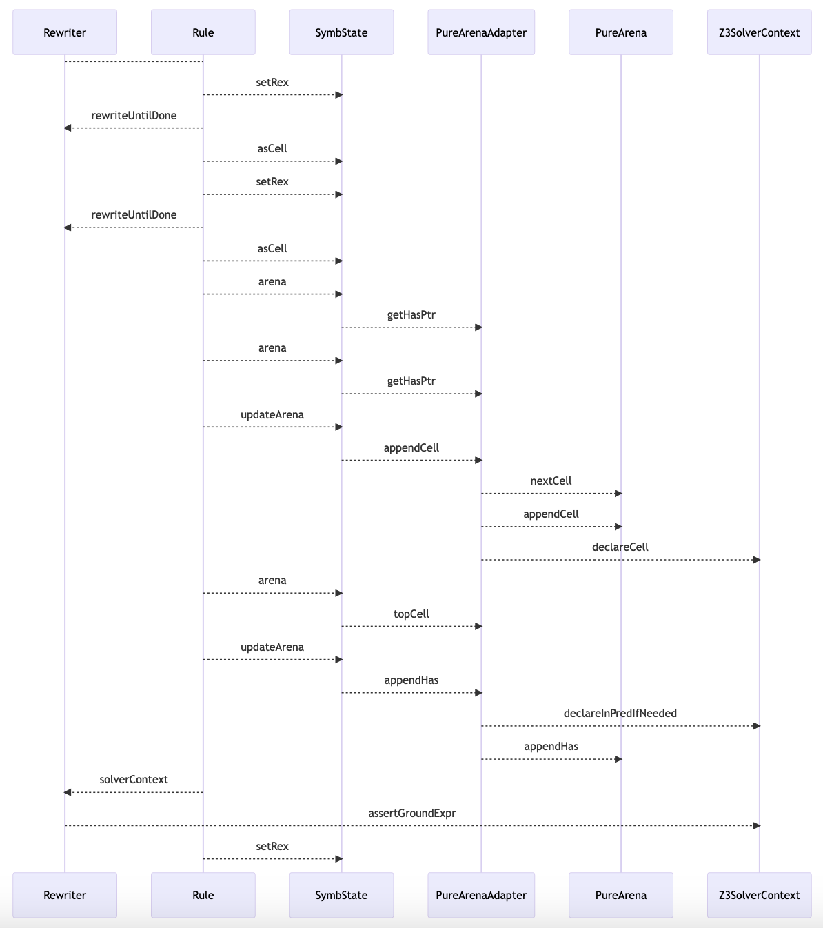
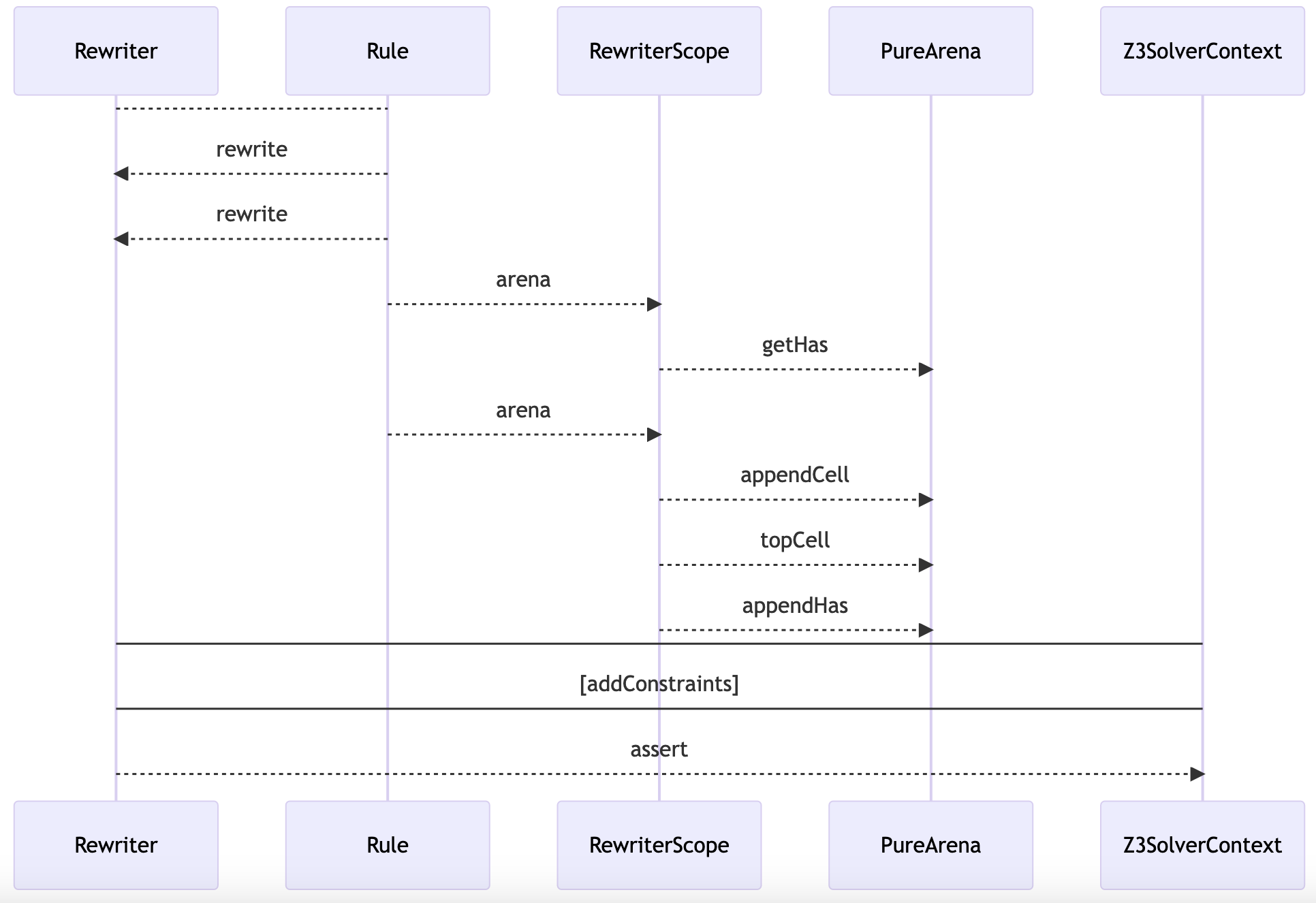
Let's have a look at the first part of this specification:
-------------------------- MODULE FoldExcept ----------------------------------
(*
 * This specification measures performance in the presence of an anti-pattern.
 *)

EXTENDS Integers, Apalache

CONSTANT
    \* A fixed set of processes
    \*
    \* @type: Set(Str);
    Proc

VARIABLES
    \* Process clocks
    \*
    \* @type: Str -> Int;
    clocks,
    \* Drift between pairs of clocks
    \*
    \* @type: <<Str, Str>> -> Int;
    drift
As we can see, the constant Proc is a specification parameter. For instance,
it can be equal to { "p1", "p2", "p3" }. The variable clocks assigns a
clock value to each process from Proc, whereas the variable drift collects
the clock difference for each pair of processes from Proc. This relation
is easy to see in the predicate Init:
The transition predicate NextFast uniformly advances the clocks of all
processes by a non-negative number delta. Simultaneously, it updates the
clock differences in the function drift.
It is easy to see that drift actually does not change between the steps. We
can formulate this observation as an action
invariant:
\* Check that the clock drifts do not change
DriftInv ==
    \A p, q \in Proc:
        drift'[p, q] = drift[p, q]
Our version of NextFast is quite concise and it uses the good parts of
TLA+. However, new TLA+ users would probably write it differently. Below, you
can see the version that is more likely to be written by a specification
writer who has good experience in software engineering:
\* Uniformly advance the clocks and update the drifts.
\* Constructing functions via explicit iteration. More like a program.
NextSlow ==
    \E delta \in Nat \ { 0 }:
        /\  LET \* @type: (Str -> Int, Str) => (Str -> Int);
                IncrementInLoop(clk, p) ==
                [ clk EXCEPT ![p] = @ + delta ]
            IN
            clocks' = ApaFoldSet(IncrementInLoop, clocks, Proc)
        /\  LET \* @type: (<<Str, Str>> -> Int, <<Str, Str>>)
                \*          => <<Str, Str>> -> Int;
                SubtractInLoop(dft, pair) ==
                LET p == pair[1]
                    q == pair[2]
                IN
                [ dft EXCEPT ![p, q] = clocks'[p] - clocks'[q] ]
            IN
            drift' = ApaFoldSet(SubtractInLoop, drift, Proc \X Proc)
The version NextSlow is less concise than NextFast, but it is probably easier to
read for a software engineer. Indeed, we update the variable clocks via
a set fold, which implements an iteration over the set of processes. What makes
it easier to understand for a software engineer is a local update in the
operator IncrementInLoop. Likewise, the variable drift is iteratively
updated with the operator SubtractInLoop.
Although NextSlow may look more familiar, it is significantly harder for
Apalache to check than NextFast. To see the difference, we measure
performance of Apalache for several sizes of Proc: 3, 5, 7, and 10. We do
this by running Apalache for the values of N equal to 3, 5, 7, 10. To this
end we define several model files called MC_FoldExcept${N}.tla for
N=3,5,7,10. For instance, MC_FoldExcept3.tla looks as follows:
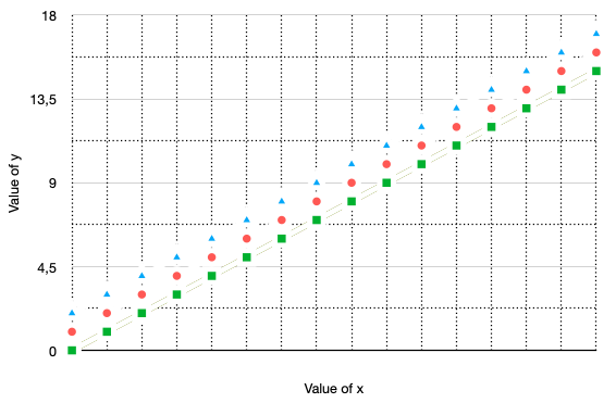
The plot below shows the running times for the versions NextSlow and
NextFast:
The plot speaks for itself. The version NextFast is dramatically faster than
NextSlow for an increasing number of processes. Interestingly, NextFast is
also more concise. In principle, both NextFast and NextSlow describe the
same behavior. However, NextFast looks higher-level: It looks like it
computes clocks and drifts in parallel, whereas NextSlow computes
these functions in a loop (though the order of iteration is unknown). Actually,
whether these functions are computed sequentially or in parallel is irrelevant
for our specification, as both NextFast and NextSlow describe a single
step of our system! We can view NextSlow as an implementation of NextFast,
as NextSlow contains a bit more computation details.
From the performance angle, the above plot may seem counterintuitive to
software engineers. Indeed, we are simply updating an array-like data structure
in a loop. Normally, it should not be computationally expensive. However,
behind the scenes, Apalache is producing constraints about all function
elements for each iteration. Intuitively, you can think of it as being fully
copied at every iteration, instead of one element being updated. From this
perspective, the iteration in NextSlow should clearly be less efficient.
A TLA+ specification defines a triple \((S,S_0,\to)\), called a transition system.
\(S\) is the state space, \(S_0\) is the set of initial states \(\left(S_0 \subseteq S\right)\),
and \(\to\) is the transition relation, a subset of \(S^2\).
The structure of a single state depends on the number of variables a specification declares.
For example, if a specification declares
VARIABLE A1, A2, A3, ..., Ak
then a state is a mapping \([A_1 \mapsto a_1, \dots, A_k \mapsto a_k]\),
where \(a_i\) represents the value of the variable Ai, for each \(i = 1,\dots,k\).
Here, we represent TLA+ variable names as unique formal symbols,
where, for example the TLA+ variable A1 is represented by the formal symbol \(A_1\).
By convention, we will use markdown-syntax to refer to objects in TLA+ specifications, and latex notation otherwise.
The state space \(S\) is then the set of all such mappings,
i.e. the set of all possible combinations of values that variables may hold.
For brevity, whenever the specification defines exactly one variable,
we will treat a state as a single value \(a_1\) instead of the mapping \([A_1 \mapsto a_1]\).
In untyped TLA+, one can think of \(S\) as \(U^{\{A_1,\dots, A_k\}}\), that is,
the set of all mappings, which assign a value in \(U\), the universe of all TLA+ values, to each symbol.
This set is naturally isomorphic to \(U^k\).
In typed TLA+, such as in Apalache, where variable declarations look like:
VARIABLE
  \* @type: T1;
  A1,
  ...,
  \* @type: Tk;
  Ak
\(S\) is additionally restricted, such that for all \(s \in S\)
each symbol \(A_i\) maps to a value \(s(A_i) \in V_i\), where \(Vi \subset U\)
is the set of all values, which hold the type \(T_i\), for each \(i = 1,\dots,k\).
For example, in the specification with
VARIABLE
  \* @type: Bool;
  A1,
  \* @type: Bool;
  A2
The state space is \(\mathbb{B}^{\{x,y\}}\) when considering types,
since each variable can hold one of two boolean values.
In the untyped setting, the state space is infinite, and contains states where,
for example, \(A1\) maps to [z \in 1..5 |-> "a"] and \(A2\) maps to CHOOSE p \in {}: TRUE.
As Apalache enforces a type system, the remainder of this document will assume the typed setting.
This assumption does not change any of the definitions.
We will also assume that every specification declares an initial-state predicate Init,
a transition-predicate Next and an invariant Inv (if not specified, assumed to be TRUE).
For simplicity, we will also assume that the specification if free of constants,
resp. that all of the constants have been initialized.
The second component, \(S_0\), the set of all initial states, is derived from \(S\) and Init.
The initial state predicate is a Boolean formula, in which specification-variables appear as free logic variables.
The operator Init characterizes a predicate \(P_{S_0} \in \mathbb{B}^S\) in the following way:
given a state \(s \in S\), the formula obtained by replacing all occurrences of variable names Ai in Init
with the values \(s(A_i)\) is a Boolean formula with no free variables (in a well-typed, parseable specification),
which evaluates to either TRUE or FALSE. We say \(P_{S_0}(s)\) is the evaluation of this formula.
By the subset-predicate equivalence, we identify the predicate \(P_{S_0}\)
with a subset \(S_0\) of \(S\): \(S_0 = \{ s \in S\mid P_{S_0}(s) = TRUE \}\).
For example, given
VARIABLE
  \* @type: Int;
  x,
  \* @type: Int;
  y

Init == x \in 3..5 /\ y = 2
we see that \(S = \mathbb{Z}^{\{x,y\}}\) and \(S_0 = \{ [x \mapsto 3, y \mapsto 2], [x \mapsto 4, y \mapsto 2], [x \mapsto 5, y \mapsto 2] \}\).
Similar to \(S_0\), \(\to\) is derived from \(S\) and Next.
If \(S_0\) is a single-argument predicate \(S_0 \in \mathbb{B}^S\),
then \(\to\) is a relation \(\to \in \mathbb{B}^{S^2}\).
\(\to(s_1,s_2)\) is the evaluation of the formula obtained by replacing all occurrences
of variable names Ai in Next with the values \(s_1(A_i)\),
and all occurrences of Ai' with \(s_2(A_i)\).
By the same principle of subset-predicate equivalence, we can treat \(\to\) as a subset of \(S^2\).
As mentioned in the notation section, it is generally more convenient to use the infix notation
\(s_1 \to s_2\) over \(\to(s_1, s_2)\). We say that a state \(s_2\)
is a successor of the state \(s_1\) if \(s_1 \to s_2\).
For example, given
VARIABLE
  \* @type: Int;
  x,
  \* @type: Int;
  y

Init == x \in 3..5 /\ y = 2

Next == x' \in { x, x + 1 } /\ UNCHANGED y
One can deduce, for any state \([x \mapsto a, y \mapsto b] \in S\), that it has two successors:
\([x \mapsto a + 1, y \mapsto b]\) and \([x \mapsto a, y \mapsto b]\)
because the following relations hold \([x \mapsto a, y \mapsto b] \to [x \mapsto a + 1, y \mapsto b]\)
and \( [x \mapsto a, y \mapsto b] \to [x \mapsto a, y \mapsto b] \).
Lastly, we define traces in the following way:
A trace of length \(k\) is simply a sequence of states \(s_0,\dots, s_k \in S\),
such that \(s_0 \in S_0\) and \(s_i \to s_{i+1}\) for all \(i\in \{0,\dots,k-1\}\).
This definition naturally extends to inifinite traces.
For example, the above specification admits the following traces of length 2 (among others):
\[
[x \mapsto 3, y \mapsto 2], [x \mapsto 3, y \mapsto 2], [x \mapsto 3, y \mapsto 2]
\]
\[
[x \mapsto 3, y \mapsto 2], [x \mapsto 4, y \mapsto 2], [x \mapsto 5, y \mapsto 2]
\]
\[
[x \mapsto 4, y \mapsto 2], [x \mapsto 5, y \mapsto 2], [x \mapsto 5, y \mapsto 2]
\]
Using the above definitions, we can define the set of states reachable in exactly \(k\)-steps,
for \(k \in \mathbb{N}\), denoted by \(R(k)\). We define \(R(0) = S_0\) and for each \(k \in \mathbb{N}\),
\[
R(k+1) := \{ t \in S \mid \exists s \in R(k) \ .\ s \to t \}
\]
Similarly, we can define the set of states reachable in at most \(k\)-steps,
denoted \(r(k)\), for \(k \in \mathbb{N}\) by
\[
r(k) := \bigcup_{i=0}^k R(i)
\]
Finally, we define the set of all reachable states, \(R\),
as the (infinite) union of all \(R(k)\), over \(k \in \mathbb{N}\):
\[
R := \bigcup_{k \in \mathbb{N}} R(k)
\]
For example, given
VARIABLE
  \* @type: Int;
  x,
  \* @type: Int;
  y

Init == x \in 1..3 /\ y = 2

Next == x' = x + 1 /\ UNCHANGED y
and so on. We can express this compactly as:
\begin{align}
[x\mapsto a, y \mapsto b] \in R(i) &\iff i+1 \le a \le i + 3 \land b = 2 \\
[x\mapsto a, y \mapsto b] \in r(i) &\iff 1 \le a \le i + 3 \land b = 2 \\
[x\mapsto a, y \mapsto b] \in R &\iff 1 \le a \land b = 2
\end{align}
We say that a transition system has a finite diameter, if there exists a \(k \in N\), such that \(R = r(k)\).
If such an integer exists then the smallest integer \(k\), for which this holds true,
is the diameter of the transition system.
In other words, if the transition system \((S,S_0,\to)\) has a finite diameter of \(k\),
any state that is reachable from a state in \(S_0\) is reachable in at most \(k\) transitions.
The example above clearly does not have a finite diameter, since \(R\) is infinite,
but \(r(k)\) is finite for each \(k\).
However, the spec
VARIABLE
  \* @type: Int;
  x

Init == x = 0

Next == x' = (x + 1) % 7
has a finite diameter (more specifically, a diameter of 6), because:
\(R = \{0,1,\dots,6\}\) (the set of remainders modulo 7), since those are the only values x',
which is defined as a % 7 expression, can take.
for any \(k = 0,\dots,5\), it is the case that \(r(k) = \{0,\dots,k\} \ne R\),
so the diameter is not in \(\{1,\dots,5\}\)
Much like Init, an invariant operator Inv defines a predicate.
However, it is not, in general, the case that Inv defines a predicate over S.
There are different cases we can consider, discussed in more detail here.
For the purposes of this document, we focus on state invariants,
i.e. operators which use only unprimed variables and no temporal- or trace- operators.
A state invariant operator Inv defines a predicate \(I\) over \(S\).
We say that the \(I\) is an invariant in the transition system, if \(R \subseteq I\), that is,
for every reachable state \(s_r \in R\), \(I(s_r)\) holds true.
If \(R \setminus I\) is nonempty (i.e., there exists a state \(s_r \in R\),
such that \(\neg I(s_r)\)), we refer to elements of \(R \setminus I\) as witnesses to invariant violation.
The goal of model checking is to determine whether or not \(R \setminus I\) contains a witness.
The goal of bounded model checking is to determine, given a bound \(k\), whether or not \(r(k) \setminus I\) contains a witness.
In a transition system with a bounded diameter, one can use bounded model checking
to solve the general model checking problem, since \(R \setminus I\) is equivalent to \(r(k) \setminus I\) for a sufficiently large \(k\). In general, if the system does not have a bounded diameter, failing to find a witness in \(r(k) \setminus I\) cannot be used to reason about the absence of witnesses in \(R \setminus I\)!
The idea behind explicit-state model checking is to simply perform the following algorithm
(in pseudocode, \(\leftarrow\) represents assignment):
Compute \(S_0\) and set \(Visited \leftarrow \emptyset, ToVisit \leftarrow S_0\)
While \(ToVisit \ne \emptyset\), pick some \(s \in ToVisit\):
1. If \(\neg I(s)\) then terminate, since a witness is found.
1. If \(I(s)\) then compute \(Successors(s) = \{ t \in S\mid s \to t \}\). Set
\begin{align}
Visited &\leftarrow Visited \cup \{s\}\\
ToVisit &\leftarrow (ToVisit \cup Successors(s)) \setminus Visited
\end{align}
If \(ToVisit = \emptyset\) terminate. \(R = Visited\) and \(I\) is an invariant.
While simple to describe, there are several limitations of this approach in practice.
The first limitation is the absence of a termination guarantee.
More specifically, this algorithm terminates if and only if \(R\) is finite.
For example:
VARIABLE
  \* @type: Int;
  x

Init == x = 0
Next == x' = x + 1
defines a state space, for which \(R = \mathbb{N}\), so the above algorithm never terminates.
Further, in the general case, it is difficult or impossible to compute \(S_0\)
or the set \(Successors(s)\) defined in the algorithm.
As an example, consider the following specification:
VARIABLE x

Successor(n) == IF n % 2 = 0 THEN n \div 2 ELSE 3*n + 1

RECURSIVE kIter(_,_)
kIter(a,k) == IF k <= 0 THEN a ELSE Successor(kIter(a, k-1))

ReachesOne(a) == \E n \in Nat: kIter(a,n) = 1

Init == x \in { n \in Nat: ~ReachesOne(n) }
The specification encodes the Collatz conjecture,
so computing \(S_0\) is equivalent to proving or disproving the conjecture,
which remains an open problem at present.
It is therefore unreasonable to expect any model checker to be able to accept such an input,
despite the fact that the condition is easily describable in first-order logic.
A similar problem can occur in computing \(Successors(s)\);
the relation between variables Ai (\(s(A_i)\)) and Ai' (\(s_2(A_i)\))
may be given by means of an implicit function or uncomputable expression.
Therefore, most tools impose the following constraints,
which make computing \(S_0\) and \(Successors(s)\) possible without any sort of specialized solver:
The specification must have the shape
or some equivalent form, in which variable values in a state can be iteratively computed,
one at a time, by means of an explicit formula, which uses only variables computed so far.
For instance,
VARIABLE x,y

Init == /\ x \in 1..0
        /\ y \in { k \in 1..10, k > x }

Next == \/ /\ x > 5
           /\ x' = x - 1
           /\ y' = x' + 1
        \/ /\ x <= 5
           /\ y' = 5 - x
           /\ x' = x + y'
allows one to compute both \(S_0\) as well as \(Successors(s)\), for any \(s\),
by traversing the conjunctions in the syntax-imposed order.
However, even in a situation where states are computable, and \(R\) is finite,
the size of \(R\) itself might be an issue in practice.
We can create very compact specifications with large state-space sizes:
Adapting the general explicit-state approach to bounded model checking is trivial,
and therefore not particularly interesting.
Assume a bound \(k \in \mathbb{N}\) on the length of the traces considered.
Compute \(S_0\) and set \(Visited \leftarrow \emptyset, ToVisit \leftarrow \{ (s,0)\mid s \in S_0 \}\)
While \(ToVisit \ne \emptyset\), pick some \((s,j) \in ToVisit\):
If \(\neg I(s)\) then terminate, since a witness is found.
If \(I(s)\) then:
\begin{align}
Visited &\leftarrow Visited \cup \{(s,j)\} \\
ToVisit &\leftarrow (ToVisit \cup T) \setminus Visited
\end{align}
where \( T \) equals \(\{(t,j+1)\mid t \in Successors(s)\}\) if \(j < k\) and \(\emptyset\) otherwise
If \(ToVisit = \emptyset\) terminate. \(r(k) = \{v \mid \exists j \in \mathbb{N} \ .\ (v,j) \in Visited\}\)
and \(I\) holds in all states reachable in at most \(k\) steps.
A real implementation would, for efficiency reasons, avoid entering the same state via traces of different length,
but the basic idea would remain unchanged.
Bounding the execution length guarantees termination of the algorithm
if \(S_0\) is finite and each state has finitely many successors w.r.t. \(\to\),
even if the state space is unbounded in general.
However, this comes at a cost of guarantees: while bounded model checking might still find an invariant violation
if it can occur within the bound \(k\), it will fail if the shortest possible trace,
on which the invariant is violated has a length greater than \(k\).
If the system has a finite diameter, bounded model checking is equivalent to model checking,
as long as \(k\) exceeds the diameter.
For a given \(k \in \mathbb{N}\), we want to find a way to determine if \(r(k) \setminus I\) is empty,
without testing every single state in \(r(k)\) like in the explicit-state approach.
The key insight behind symbolic model checking is the following:
it is often the case that the size of the reachable state space is large,
not because of the properties of the specification, but simply because of the constants or sets involved.
Consider the example:
VARIABLE
  \* @type: Int;
  x

Init == x = 1
Next1 == x' \in 1..9
Next2 == x' \in 1..999999999999

Inv == x < 5
The sets of reachable states defined by each Next have sizes proportional to the upper bounds of the ranges used.
However, to find a violation of the invariant, one merely needs to identify a state \(s\)
in which, for example, \(s(x) = 7\), which belongs to both sets.
It is not necessary, or efficient, to loop over elements in the range and test each one against Inv to find a violation.
Depending on the logic fragment Inv belongs to, there usually exist strategies for finding such violations much faster.
From this perspective, if, for some \(k\), we succeeded in finding a predicate \(P\) over \(S\), such that:
\(P\) belongs to a logic fragment, for which optimizations exist
\(P\) has a witness iff a state reachable in at most \(k\) steps violates \(I\): \(\left(\exists s \in S \ .\ P(s)\right) \iff r(k) \setminus I \ne \emptyset\)
we can use specialized techniques within the logical fragment to evaluate \(P\)
and find a witness to the violation of \(I\), or else conclude that \(r(k) \subseteq I\).
To do this, it is sufficient to find a predicate \(P_R^l\) encoding \(R(l)\),
for each \(l \in \{0,\dots,k\}\), since:
\begin{align}
s \in r(l) \iff& \lor s \in R(0) \\
&\lor s \in R(1) \\
&\dots \\
&\lor s \in R(l)
\end{align}
How does one encode \(P_R^0\)?
\[
s \in R(0) \iff s \in S_0 \iff P_{S_0}(s)
\]
so \(P_R^0(s) = P_{S_0}(s)\). What about \(P_R^1\)?
\begin{align}
s \in R(1) &\iff s \in \{ t \in S \mid \exists s_0 \in R(0) \ .\ s_0 \to t \} \\
&\iff \exists s_0 \in R(0) \ .\ s_0 \to s \\
&\iff \exists s_0 \in S \ .\ P_R^0(s_0) \land s_0 \to s
\end{align}
so \(P_R^1(s) := \exists s_0 \in S \ .\ P_R^0(s_0) \land s_0 \to s\)
continuing this way, we can determine
\[
P_R^k(s) := \exists s_{k-1} \in S \ .\ P_R^{k-1}(s_{k-1}) \land s_{k-1} \to s
\]
Which can be expanded to
\[
Pk(s) = \exists s_0,\dots,s_{k-1} \in S \ .\ P_{S_0}(s_0) \land s_0 \to s_1 \land s_1 \to s_2 \land \dots \land s_{k-1} \to s
\]
Then, the formula describing invariant violation in exactly \(k\) steps, \(\exists s_k \in R(k) \setminus I\), becomes
\[
\exists s_0,\dots,s_k \in S \ .\ P_{S_0}(s_0) \land \neg I(s_k) \land \bigwedge_{i=0}^{k-1} s_i \to s_{i+1}
\]
The challenge in designing a symbolic model checker is determining, given TLA+ operators Init, Next and Inv,
the encodings of \(P_{S_0}, \to, I\) as formulas in logics supported by external solvers, for example SMT.
In an explicit approach, the basic unit of computation is a single state \(s \in S\).
However, as demonstrated above, symbolic approaches deal with logical formulas.
Recall that a state formula, such as Init is actually a predicate over \(S\),
and a predicate is equivalent to a subset of \(S\).
Predicates tend to not distinguish between certain concrete states. For instance, the formula
\(x < 3\) is equally false for both \(x = 7\) and \(x = 70000000\).
It is useful to characterize all of the states, in which a predicate evaluates to the same value.
This is because we will define symbolic states in terms of equivalence relations:
A predicate \(P\) over \(S\) naturally defines an equivalence relation \(\circledcirc_P\):
For \(a,b \in S\), we say that \(a \circledcirc_P b\) holds if \(P(a) = P(b)\).
Proving that this relation satisfies the criteria for an equivalence relation is left as an exercise to the reader.
This equivalence relation has only two distinct equivalence classes, since \(P(s)\) can only be TRUE or FALSE.
We can therefore think of predicates in the following way: Each predicate \(P\) slices the
set \(S\) into two disjoint subsets, i.e. the equivalence classes of \(\circledcirc_P\).
An equivalent formulation of the above is saying that each predicate \(P\)
defines a quotient space \(S / \circledcirc_P\), of size \(2\).
Recall that we have expressed the set of states \(R(l)\) with the predicate \(P_R^l\),
for each \(l \in \{0,\dots,k\}\). By the above, \(P_R^l\) defines an equivalence relation
\(\circledcirc_{P_R^l}\) on \(S\), and consequently, two equivalence classes.
For notational clarity, we use \(\circledcirc^l\) instead of \(\circledcirc_{P_R^l}\).
Each concrete state \(s \in S\) belongs to exactly one equivalence class \(\lbrack s \rbrack_{ \circledcirc^l} \in S / \circledcirc^l\).
The states in \(R(l)\) correspond to the equivalence class in which \(P_R^l\)
holds true (i.e. \(s \in R(l) \iff \lbrack s \rbrack_{\circledcirc^l} = \{t \in S \mid P_R^l(t) = TRUE\}\)),
and the ones in \(S \setminus R(l)\) correspond to the equivalence class in which \(P_R^l\) is false
(i.e. \(s \notin R(l) \iff \lbrack s \rbrack_{\circledcirc^l} = \{t \in S \mid P_R^l(t) = FALSE\}\)).
We define symbolic states in the following way: Given a predicate \(P\) over \(S\),
a symbolic state with respect to \(P\) is an element of \(S / \circledcirc_P\),
where \(\circledcirc_P\) is the equivalence relation derived from \(P\) (i.e. \(a \circledcirc_P b \iff P(a) = P(b)\)).
Recall the subset-predicate equivalence: in this context, a symbolic state, w.r.t. \(P\)
is equivalent to a predicate, specifically, either \(P\) or \(\neg P\).
For example, given
VARIABLE
  \* @type: Int;
  x,
  \* @type: Int;
  y


Init == x = 1 /\ y = 1
Next == x' \in 1..5 /\ y \in {0,1}
and the predicate \(P(s) = s(x) < 3\), the symbolic states are
\[
\{ [x \mapsto a, y \mapsto b] \mid a,b\in \mathbb{Z} \land a < 3 \}
\]
and
\[
\{ [x \mapsto a, y \mapsto b] \mid a,b\in \mathbb{Z} \land a \ge 3 \}
\]
while the symbolic states w.r.t. \(R(0)\) are
\[
\{ [x \mapsto 1, y \mapsto 1] \}
\]
and
\[
\{ [x \mapsto a, y \mapsto b] \mid a,b\in \mathbb{Z} \land ( a \ne 1 \lor b \ne 1 )\}
\]
If we only care about characterizing invariant violations, the above techniques are sufficient.
However, specification invariants are often composed of multiple smaller, independent invariants.
For feedback purposes, it can be beneficial to identify, whenever an invariant violation occurs,
the precise sub-invariant that is the cause.
Suppose we are given an invariant \(s(x) > 0 \land s(y) > 0\).
The information whether a reachable state has just \(s(x) \le 0\), just \(s(y) \le 0\),
or both can help determine problems at the design level.
More generally: often, a predicate \(P\) is constructed as a conjunction of other predicates,
e.g. \(P(s) \iff p_1(s) \land \dots \land p_m(s)\). A violation of \(P\) means a violation of (at least) one of
\(p_1,\dots,p_m\), but knowing which one enables additional analysis.
A collection of predicates \(p_1,\dots,p_m\) over \(S\) define an equivalence relation
\(\circledcirc\lbrack p_1,\dots,p_m\rbrack\)in the following way:
For \(a,b \in S\), we say that \( a \circledcirc\lbrack p_1,\dots,p_m\rbrack\ b\) holds if
\(p_1(a) = p_1(b) \land \dots \land p_m(a) = p_m(b)\).
Clearly, \(\circledcirc\lbrack p_1\rbrack = \circledcirc_{p_1}\).
Since a predicate can only evaluate to one of two values, there exist only two equivalence classes for
\(\circledcirc_P\), i.e. only two symbolic states w.r.t. \(P\): one is the set of all states for which
\(P\) is TRUE, and the other is the set of all values for which \(P\) is FALSE.
In this sense, \(S / \circledcirc_P\) is isomorphic to the set \(\mathbb{B}\).
In the case of \(\circledcirc\lbrack p_1,\dots,p_m\rbrack\), there are \(2^m\) different \(m\)-tuples with values from
\(\mathbb{B}\), so \(S / \circledcirc\lbrack p_1,\dots,p_m\rbrack\) is isomorphic to \(\mathbb{B}^m\) .
What is the relation between \(\circledcirc\lbrack p_1,\dots,p_m\rbrack\) and \(\circledcirc_P\),
where \(P(s) = p_1(s) \land \dots \land p_m(s)\)?
Clearly, \(P(s) = TRUE \iff p_1(s) = \dots = p_m(s) = TRUE\).
Consequently, there is one equivalence class in \(S / \circledcirc_P\), that is equal to
\[
C_1 = \{ s \in S \mid P(s) = TRUE \}
\]
and one equivalence class in \(S / \circledcirc\lbrack p_1,\dots,p_m\rbrack\) that is equal to
\[
C_2 = \{ s \in S \mid p_1(s) = TRUE \land \dots \land p_m(s) = TRUE \}
\]
They are one and the same, i.e. \(C_1 = C_2\). The difference is, that splitting \(P\) into \(m\) components
\(p_1,\dots,p_m\) splits the other (unique) equivalence class \(C \in \{ c \in S / \circledcirc_P \mid c \ne C_1 \}\)
into \(2^m - 1\) parts, which are the equivalence classes in \(\{ c \in S/\circledcirc\lbrack p_1,\dots,p_m\rbrack \mid c \ne C_2 \}\).
Consequently, we can also define symbolic states with respect to a set of predicates \(p_1,\dots,p_m\),
implicitly conjoined, as elements of \(S / \circledcirc\lbrack p_1,\dots,p_m\rbrack\).
Similarly, by the subset-predicate equivalence, a symbolic state, w.r.t. \(p_1,\dots,p_m\) can be viewed as one of
\begin{align}
p_1(s) \land p_2(s) \land \dots \land p_m(s) \qquad&= P(s) \\
\neg p_1(s) \land p_2(s) \land \dots \land p_m(s) \qquad& | \\
p_1(s) \land \neg p_2(s) \land \dots \land p_m(s) \qquad& | \\
\dots \qquad& |> \text{(as a disjunction)} = \neg P(s) \\
\neg p_1(s) \land \neg p_2(s) \land \dots \land \neg p_{m-1}(s) \land p_m(s) \qquad& | \\
\neg p_1(s) \land \neg p_2(s) \land \dots \land \neg p_{m-1}(s) \land \neg p_m(s) \qquad& | \\
\end{align}
For example, take \(p_1(s) = s \in R(k)\) and \(p_2(s) = \neg I(s)\). With respect to \(p_1(s) \land p_2(s)\),
there are two symbolic states: one corresponds to the set of all states which are both reachable and in which the invariant is violated,
while the other corresponds to the set of all states, which are either not reachable, or in which the invariant holds.
Conversely, with respect to \(p_1,p_2\), there are four symbolic states: one corresponds to states
which are both reachable and violate the invariant, one corresponds to states which are reachable,
but which do not violate the invariant, one corresponds to states which are not reachable,
but violate the invariant and the last one corresponds to states which are neither reachable, nor violate the invariant.
Having defined symbolic states, what is then the meaning of a symbolic trace?
Recall, a trace of length \(k\) is simply a sequence of reachable states
\(s_0,\dots, s_k \in S\), such that \(s_0 \in S_0\) and \(s_i \to s_{i+1}\).
In the symbolic setting, a symbolic trace is a sequence of symbolic states \(C_0,\dots,C_k \subseteq S\), such that
\[
C_0 \in S / \circledcirc^0 \land \dots \land C_k \in S / \circledcirc^k
\]
and, for each \(i = 0,\dots,k\), it is the case that \(C_i = \{ s \in S \mid P_R^i(s) = TRUE\}\).
In other words, a symbolic trace is the unique sequence of symbolic states, which correspond to the set
of explicit states evaluating to TRUE under each of \(P_R^0,\dots,P_R^k\) respectively.
Recall that \(P_R^{i+1}(s_{i+1})\) was defined as \(\exists s_i \in S \ .\ P_R^i(s_i) \land s_i \to s_{i+1}\).
While, in the explicit case, we needed to enforce the condition \(s_i \to s_{i+1}\),
in the symbolic case this is already a part of the predicate definition.
For example, consider:
VARIABLE
  \* @type: Int;
  x

Init == x \in {0,1}
Next == x' = x + 1
a trace of length 2 would be one of \(0,1,2\) or \(1,2,3\). A symbolic trace would be the sequence
\[
\{0,1\}, \{1,2\}, \{2,3\}
\]
In the case of symbolic states, we were particularly interested in symbolic states with respect to predicates that encoded reachability.
Unlike the case of invariants, where we considered conjunctions of sub-invariants,
the most interesting scenario w.r.t. traces is when a transition relation is presented as a disjunction of transitions,
i.e. when
\begin{align}
s_1 \to s_2 \iff& \lor t_1(s_1,s_2)\\
& \lor t_2(s_1,s_2)\\
& \dots \\
& \lor t_m(s_1,s_2)
\end{align}
At the specification level, this is usually the case when one can nondeterministically choose to perform one of \(m\) actions,
and each \(t_1,\dots,t_m\) is an encoding of one such action, which, like \(\to\), translates to a binary predicate over \(S\).
Instead of a single trace \(C_1, \dots, C_k\), where states in \(C_{i+1}\) are reachable from states in
\(C_i\) via \(\to\), we want to separate sets of states reachable by each \(t_i\) individually.
Recall that symbolic traces are sequences of symbolic states, implicitly related by \(\to\),
since \(R\) is defined in terms of \(\to\).
We define a symbolic trace decomposition by \(t_1,\dots,t_m\), in the following way:
If \(t_1,\dots,t_m\) are relations, such that \(s_1 \to s_2 \iff \bigvee_{i=1}^m t_i(s_1,s_2)\),
the decomposition of a symbolic trace \(X_0,\dots,X_k\) of length \(k\) w.r.t. \(t_1,\dots,t_m\) is a set \(
D = \{
Y(\tau) \mid \tau \in \{1,\dots,m\}^{\{1,\dots, k\}}
\}
\) , such that:
\(Y(\tau)\) is a partial symbolic trace of length k: \(Y_0(\tau) = X_0, Y_1(\tau),\dots, Y_k(\tau)\)
For each \(i = 0,\dots,k-1\), \(Y_{i+1}\) is the set of all states reachable from \(Y_i\) by the transition fragment \(t_j\), where \(j = \tau(i+1)\):
\[
Y_{i+1}(\tau) = \{ s_{i+1} \in X_{i+1} \mid \exists s_i \in Y_i(\tau) \ .\ t_{\tau(i+1)}(s_i,s_{i+1}) \}
\]
An interesting property to observe is that, for each \(i=1,\dots,k\), the sets
\(Y_i(\tau)\), over all possible \(\tau\), form a decomposition of \(X_i\). Concretely:
\[
X_i = \bigcup \left\{ Y_i(\tau)\mid \tau \in \{1,\dots,m\}^{\{1,\dots, k\}} \right\}
\]
Less obvious is the fact that, the larger the index \(i\), the finer this decomposition becomes.
Consider \(i=1\). Since \(Y_0\) is fixed, there are as many different \(Y_1(\tau)\) components as there are possible values of
\(\tau(1)\), i.e. \(m\). As \(Y_2\) depends on \(Y_1\), there are as many different components as there are pairs
\((\tau(1),\tau(2))\), i.e. \(m^2\), and so on until \(k\), where there are \(m^k\) possible \(Y_k(\tau)\) sets.
In practice, however, many of these sets are empty.
Let us look at an example:
VARIABLE
  \* @type: Int;
  x

A1 == /\ x > 4
      /\ x' = x - 1

A2 == /\ x < 7
      /\ x' = x + 1

A3 == x' = x

A4 == /\ x = 1
      /\ x' = 10

Init == x \in 1..10
Next == \/ A1
        \/ A2
        \/ A3
        \/ A4
Suppose we fix the length of the trace \(k = 2\).
Without considering the decomposition, the symbolic trace is equal to
\[
X_0 = \{1,\dots,10\}, X_1 = \{1,\dots,10\}, X_2 = \{1,\dots,10\}
\]
Under the decomposition, we have \(m^k = 4^2 = 16\) candidates for \(\tau\).
Let us look at \(\tau_1\), for which \(\tau_1(1) = 1, \tau_1(2) = 2\), representing an execution
where the action A1 is followed by the action A2.
If \(Y_0(\tau_1),Y_1(\tau_1),Y_2(\tau_1)\) is a partial trace (i.e. one of the elements in the decomposition \(D\)),
then:
\(Y_1(\tau_1) = \{ b \in X_1 \mid \exists a \in Y_0(\tau_1) \ .\ t_{\tau_1(1)}(a,b)\}\) which means
\[
Y_1(\tau_1) = \{ b \in \{1,\dots,10\} \mid \exists a \in \{1,\dots,10\} \ .\ a > 4 \land b = a - 1 \}
= \{4,\dots,9\}
\]
\(Y_2(\tau_1) = \{ b \in X_2 \mid \exists a \in Y_1(\tau_1)\ .\ t_{\tau_1(2)}(a,b)\}\) which means
\[
Y_2(\tau_1) = \{ b \in \{1,\dots,10\} \mid \exists a \in \{4,\dots,9\} \ .\ a < 7 \land b = a + 1 \}
= \{5,\dots,7\}
\]
so the partial trace, corresponding to the sequence of actions Init,A1,A2 is
\[
\{1,\dots,10\}, \{4,\dots,9\}, \{5,\dots,7\}
\]
In fact, we can draw a table, representing partial traces corresponding to sequences of actions:
Sequence of actions (after Init)
Partial trace (without \(Y_0\))
A1, A1
\(\{4, \dots, 9\}, \{4, \dots, 8\}\)
A1, A2
\(\{4, \dots, 9\}, \{5, \dots, 7\}\)
A1, A3
\(\{4, \dots, 9\}, \{4, \dots, 9\}\)
A1, A4
\(\{4, \dots, 9\}, \emptyset\)
A2, A1
\(\{2, \dots, 7\}, \{4, \dots, 6\}\)
A2, A2
\(\{2, \dots, 7\}, \{3, \dots, 7\}\)
A2, A3
\(\{2, \dots, 7\}, \{2, \dots, 7\}\)
A2, A4
\(\{2, \dots, 7\}, \emptyset\)
A3, A1
\(\{1, \dots, 10\}, \{4, \dots, 9\}\)
A3, A2
\(\{1, \dots, 10\}, \{2, \dots, 7\}\)
A3, A3
\(\{1, \dots, 10\}, \{1, \dots, 10\}\)
A3, A4
\(\{1, \dots, 10\}, \{10\}\)
A4, A1
\(\{10\}, \{9\}\)
A4, A2
\(\{10\}, \emptyset\)
A4, A3
\(\{10\}, \{10\}\)
A4, A4
\(\{10\}, \emptyset\)
Clearly, the elements in every column (representing the various \(Y_i(\tau)\)), add up to \(X_i = \{1,\dots,10\}\).
Also noticeable is the fact that some actions disable others, represented by the fact that some \(Y_2(\tau)\) sets are empty.
For example, the action A2 disables A4, because after A2, x cannot hold the value \(1\), which is a precondition for A4.
Finally, we can interpret Apalache counterexamples in the context of the above definitions.
Given an invariant \(I\), a transition system \((S, S_0, \to)\) and an upper bound on executions \(k\),
Apalache first finds predicates \(t_1,\dots,t_m\) partitioning \(\to\).
Then, it encodes a symbolic trace \(X_0,\dots,X_k\) and its decomposition \(D\).
A counterexample in Apalache defines an explicit trace \(s_0,s_1,\dots,s_l \in S\) for some \(l \le k\),
as well as a sequence \(t_{\tau(1)}, \dots, t_{\tau(l)}\) (in the comments).
The predicate sequence defines a partial trace (of length \(l\))
\(Y_0(\tau),\dots,Y_l(\tau)\) and \(s_0,\dots,s_l\) are chosen such that \(s_i \in Y_i(\tau)\).
Take the following specification and counterexample, for \(k = 10\):
---------- MODULE example ----------

EXTENDS Integers

VARIABLE
  \* @type: Int;
  x

A == /\ x = 1
     /\ x' = x + 1
B == /\ x > 1
     /\ x' = x + 1

Init == x = 1
Next == \/ A
        \/ B
Inv == x < 3

====================

---------------------------- MODULE counterexample ----------------------------

EXTENDS test

(* Constant initialization state *)
ConstInit == TRUE

(* Initial state *)
State0 == x = 1

(* Transition 0 to State1 *)
State1 == x = 2

(* Transition 1 to State2 *)
State2 == x = 3

(* The following formula holds true in the last state and violates the invariant *)
InvariantViolation == x >= 3

================================================================================
We can see that, even though \(k=10\), we found a violation in \(l=2\) steps.
Each State{i} represents one of \(s_0,\dots,s_l\), by explicitly defining variable values in that state (e.g. x = 1 /\ y = 2 /\ z = "A").
The comment (* Transition X to StateY *) outlines which \(t_1,\dots,t_m\) was used to reach \(s_{i+1}\) from \(s_i\) (0-indexed).
The shape of \(t_i\) can be found by looking at the file XX_OutTransitionFinderPass.tla, and will be named Next_si_i.
In the above case, Transition 0 refers to the one representing A and Transition 1 refers to the one representing B.
InvariantViolation is the negation of the invariant Inv, and it will hold in State{l} (in this case, x < 3 does not hold in State2, where x = 3).
Common sets: We use the notation \(\mathbb{Z}\) to refer to the set of all integers, \(\mathbb{B}\)
to refer to the set of Booleans \(\{TRUE,FALSE\}\), and \(\mathbb{N}\) to refer to the set of all naturals,
i.e. \(\mathbb{N} = \{z \in \mathbb{Z}\mid z \ge 0\}\).
Function sets: We denote by \(B^A\) the set of all functions from \(A\) to \(B\), i.e. \(f \in B^A \iff f\colon A \to B\).
Powersets: We denote by \(2^A\) the set of all subsets of a set \(A\), i.e.
\(B \subseteq A \iff B \in 2^A\)
Isomorphisms: Sets \( A \) and \(B\) are called isomorphic, if there exists a bijective function
\(b\in B^A\).
Predicates: Given a set \(T\), a predicate over \(T\) is a function \(P \in \mathbb{B}^T\), that is,
a function \(P\), such that \(P(t) \in \mathbb{B}\) for each \(t \in T\).
Relations: Predicates over \(A \times B\) are called relations. A relation \(R\) over \(T \times T\) is an equivalence relation,
if the following holds:
For all \(t \in T\), it is the case that \(R(t,t)\) (reflexivity).
For all \(s,t \in T\), \(R(s,t)\) holds if and only if \(R(t,s)\) holds (symmetry).
For all \(r,s,t \in T\), \(R(r,s) \land R(s,t)\) implies \(R(r,t)\) (transititvity).
Equivalence classes: An equivalence relation \(R\) over \(T \times T\) defines a function \(E \in (2^T)^T\),
such that, for each \(t \in T\), \(E(t) = \{ s \in T\mid R(t,s) \}\). \(E(t)\)
is called the equivalence class of \(t\) for \(R\), denoted as \(\lbrack t\rbrack_R\).
Quotient space: An equivalence relation \(R\) over \(T \times T\) defines a quotient space, denoted \(T / R\),
such that \(T / R = \{ \lbrack t\rbrack_R \mid t \in T \} \subseteq 2^T\).
Subset-predicate equivalence: For any set \(T\), there exists a natural isomorphism between
\(\mathbb{B}^T\) and \(2^T\) (implied by the similarity in notation): Each predicate \(P \in \mathbb{B}^T\)
corresponds to the set \(\{ t \in T \mid P(t) = TRUE\} \in 2^T\).
For this reason, predicates are often directly identified with the subset they are equivalent to, and we write \(P \subseteq T\) for brevity.
Infix notation: Given a relation \(R \in \mathbb{B}^{A\times B}\), we commonly write \(a\ R\ b\)
instead of \(R(a,b)\) (e.g. \(a > b\) instead of \(>(a,b)\)).
Cartesian product: Given a set \(T\), we use \(T^2\) to refer to \(T \times T\).
\(T^k\), for \(k > 2\) is defined similarly.
In this tutorial, we will show how Apalache can be used to decide temporal
properties that are more general than invariants.
This tutorial will be most useful to you if you have a basic understanding of
linear temporal logic, e.g. the semantics of <> and [] operators.
See a writeup of temporal operators here.
Further, we assume you are familiar with TLA+, but expert knowledge is not necessary.
As a running example, the tutorial uses a simple example specification, modelling a
devious nondeterministic traffic light.
The traffic light has two main components: A lamp which can be either red or green,
and a button which can be pushed to request the traffic light to become green.
Consequently, there are two variables:
the current state of the light (either green or red),
and whether the button has been pushed that requests the traffic light to switch from red to green.
The full specification of the traffic light is here:
TrafficLight.tla.
But don't worry - we will dissect the spec in the following.
In the TLA specification, we declare two variables:
VARIABLES
    \* If true, the traffic light is green. If false, it is red.
    \* @type: Bool;
    isGreen,

    \* If true, the button has been pushed to request the light to become green, but the light has
    \* not become green since then.
    \* If false, the light has become green since the button has last been pushed
    \* or the button has never been pushed.
    \* @type: Bool;
    requestedGreen
Initially, the light is red and green has not yet been requested:
\* The light is initially red, and the button was not pressed.
Init ==
    /\ isGreen = FALSE
    /\ requestedGreen = FALSE
We have three possible actions:
The traffic light can switch from red to green,
The traffic light can switch from green to red, or
The button can be pushed, thus requesting that the traffic light becomes green.
(* ---------------------- *)
(* requesting green light *)
\* The switch to green can only be requested when the light is not green, and
\* the switch has not *already* been requested since the light last turned green.
RequestGreen_Guard ==
    /\ ~isGreen
    /\ ~requestedGreen

RequestGreen_Effect ==
    /\ requestedGreen' = TRUE
    /\ UNCHANGED << isGreen >>

RequestGreen ==
    RequestGreen_Guard /\ RequestGreen_Effect

(* ---------------------- *)
(* switching to red light *)
\* The light can switch to red at any time if it is currently green.
SwitchToRed_Guard == isGreen

SwitchToRed_Effect ==
    /\ isGreen' = FALSE
    /\ UNCHANGED << requestedGreen >>

SwitchToRed ==
    SwitchToRed_Guard /\ SwitchToRed_Effect

(* ------------------------ *)
(* switching to green light *)
\* The light can switch to green if it is currently red, and
\* the button to request the switch to green has been pressed.
SwitchToGreen_Guard ==
    /\ ~isGreen
    /\ requestedGreen

SwitchToGreen_Effect ==
    /\ isGreen' = TRUE
    /\ requestedGreen' = FALSE

SwitchToGreen ==
    SwitchToGreen_Guard /\ SwitchToGreen_Effect

Next ==
    \/ RequestGreen
    \/ SwitchToRed
    \/ SwitchToGreen
In the interest of simplicity, we'll assume that
the button cannot be pushed when green is already requested, and
that similarly it's not possible to push the button when the light is
already green.
Now, we are ready to specify the properties that we are interested in.
For example, when green is requested, at some point afterwards the light should actually turn green.
We can write the property like this:
Intuitively, the property says:
"Check that at all points in time ([]),
if right now, RequestGreen is true,
then at some future point in time, IsGreen is true."
...
The outcome is: NoError
Checker reports no error up to computation length 10
It took me 0 days  0 hours  0 min  2 sec
Total time: 2.276 sec
EXITCODE: OK
This is because our traffic watch is actually
deterministic:
If it is red and green has not been requested,
the only enabled action is RequestGreen.
If it is red and green has been requested,
only SwitchToGreen is enabled.
And finally, if the light is green,
only SwitchToRed is enabled.
However, we want to make our traffic light more devious.
We will allow the model to stutter, that is,
just let time pass and take no action.
We can write a new next predicate that explicitly allows
stuttering like this:
Step 2: picking a transition out of 3 transition(s)               I@18:04:16.132
State 3: Checking 1 state invariants                              I@18:04:16.150
State 3: Checking 1 state invariants                              I@18:04:16.164
State 3: Checking 1 state invariants                              I@18:04:16.175
State 3: Checking 1 state invariants                              I@18:04:16.186
Check an example state in: /home/user/apalache/docs/src/tutorials/_apalache-out/TrafficLight.tla/2022-05-30T18-04-13_3349613574715319837/counterexample1.tla, /home/user/apalache/docs/src/tutorials/_apalache-out/TrafficLight.tla/2022-05-30T18-04-13_3349613574715319837/MC1.out, /home/user/apalache/docs/src/tutorials/_apalache-out/TrafficLight.tla/2022-05-30T18-04-13_3349613574715319837/counterexample1.json, /home/user/apalache/docs/src/tutorials/_apalache-out/TrafficLight.tla/2022-05-30T18-04-13_3349613574715319837/counterexample1.itf.json E@18:04:16.346
State 3: state invariant 0 violated.                              E@18:04:16.346
Found 1 error(s)                                                  I@18:04:16.347
The outcome is: Error                                             I@18:04:16.353
Checker has found an error                                        I@18:04:16.354
It took me 0 days  0 hours  0 min  2 sec                          I@18:04:16.354
Total time: 2.542 sec                                             I@18:04:16.354
This time, we get a counterexample.
Let's take a look at /home/user/apalache/docs/src/tutorials/_apalache-out/TrafficLight.tla/2022-05-30T18-04-13_3349613574715319837/counterexample1.tla.
The initial state formula appears twice, once as a comment and once in TLA+.
There are way more variables than the two variables we specified.
The comment and the TLA+ specification express the same state, but in the comment,
some variable names from the encoding have been replaced with more human-readable names.
For example, there is a variable called ☐(requestedGreen ⇒ ♢isGreen) in the comment,
which is called __temporal_t_1 in TLA+.
In the following, let's focus on the content of the comment, since it's easier to understand what's going on.
There are many additional variables in the counterexample, because to check temporal formulas, Apalache uses an
encoding that transforms temporal properties to invariants.
If you are interested in the technical details, the encoding is described in sections 3.2 and 4 of Biere et al..
However, to understand the counterexample, you don't need to go into the technical details of the encoding.
We'll go explain the counterexample in the following.
We will talk about traces in the following.
You can find more information about (symbolic) traces here.
For the purpose of this tutorial, however, it will be enough to think of a trace as a sequence of states
that were encountered by Apalache, and that demonstrate a violation of the property that is checked.
First, it's important to know that for finite-state systems, counterexamples to temporal properties are traces ending in a loop,
which we'll call lassos in the following. If you want to learn more about why this is the case,
have a look at the book on model checking.
A loop is a partial trace that starts and ends with the same state.
A lasso is made up of two parts: A prefix, followed by a loop.
It describes a possible infinite execution: first it goes through the prefix, and then repeats the loop forever.
For example, what is a trace that is a counterexample to the property ♢isGreen?
It's an execution that loops without ever finding a state that satisfies isGreen.
For example, a counterexample trace might visually look like this:
In contrast, as long as the model checking engine has not found a lasso, there may still exist some future state satisfying isGreen.
The encoding for temporal properties involves lots of auxiliary variables.
While some can be very helpful to understand counterexamples,
many are mostly noise.
Let's first understand how Apalache can identify lassos using auxiliary variables.
The auxiliary variable __loop_InLoop is true in exactly the states belonging to the loop.
Additionally, at the first state of the loop, i.e., when __loop_InLoop switches from false to true,
we store the valuation of each variable in a shadow copy whose name is prefixed by __loop_.
Before the first state of the loop, the __loop_ carry arbitrary values.
In our example, it looks like this:
So, initially, isGreen and requestedGreen are both false.
Further, __loop_InLoop is false, and the copies of isGreen and requestedGreen, which are called
__loop_isGreen and __loop_requestedGreen, are equal to the values of isGreen and requestedGreen.
From state 0 to state 1, requestedGreen changes from false to true.
From state 1 to state 2, the system stutters, and the valuation of model variables remains unchanged.
Finally, in state 3 __loop_InLoop is set to true, which means that
the loop starts in state 2, and the trace from state 3 onward is inside the loop.
However, since state 3 is the last state, this means simply that the trace loops in state 2.
Since the loop starts, the copies of the system variables are also set to the values of the variables in state 2,
so __loop_isGreen = FALSE and __loop_requestedGreen = TRUE.
The lasso in this case can be visualized like this:
It is also clear why this trace violates the property:
requestedGreen holds in state 1, but isGreen never holds,
so in state 1 the property requestedGreen => <>isGreen is violated.
Next, let us discuss the other auxiliary variables that are introduced by Apalache to check the temporal property.
These extra variables correspond to parts of the temporal property we want to check.
These are the following variables with their valuations in the initial state:
Variables that look like formulas, e.g. ☐(requestedGreen ⇒ ♢isGreen)
Variables that look like formulas and end with _unroll,
e.g. ☐(requestedGreen ⇒ ♢isGreen)_unroll
The variable RequestWillBeFulfilled_init.
Let's focus on the non-_unroll variables that look like formulas
first.
Recall that the temporal property we want to check is [](requestedGreen => <>isGreen).
That's also the name of one of the variables: The value of the variable
☐(requestedGreen ⇒ ♢isGreen) tells us whether starting in the current state, the
formula [](requestedGreen => <>isGreen) holds. Since we are looking at a counterexample to this formula, it is not
surprising that the formula does not hold in the initial state of the counterexample.
Similarly, the variable requestedGreen ⇒ ♢isGreen tells us whether
the property requestedGreen ⇒ ♢isGreen holds at the current state.
It might be surprising to see that the property holds
but recall that in state 0, requestedGreen = FALSE, so the implication is satisfied.
Finally, we have the variable ♢isGreen, which is false, telling
us that along the execution, isGreen will never be true.
You might already have noticed the pattern of which formulas appear as variables.
Take our property [](requestedGreen => <>isGreen).
The syntax tree of this formula looks like this:
For each node of the syntax tree where the formula contains a temporal operator,
there is an auxiliary variable.
For example, there would be auxiliary variables for the formulas []isGreen
and (<>isGreen) /\ ([]requestedGreen), but not for the formula isGreen /\ requestedGreen.
As mentioned before, the value of
an auxiliary variable in a state tells us whether from that state, the corresponding subformula is true.
In this particular example, the formulas that correspond to variables in the encoding are filled with orange in the syntax tree.
What about the _unroll variables? There is one _unroll variable for each immediate application of a temporal operator in the formula.
For example, ☐(requestedGreen ⇒ ♢isGreen)_unroll is the unroll-variable for the
leading box operator.
To illustrate why these are necessary, consider the formula
[]isGreen. To decide whether this formula holds in the last state of the loop, the algorithm needs to know whether
isGreen holds in all states of the loop. So it needs to store this information when it traverses the loop.
That's why there is an extra variable, which stores whether isGreen holds on all states of the loop,
and Apalache can access this information when it explores the last state of the loop.
Similarly, the unroll-variable ♢isGreen_unroll holds true
if there is a state on the loop such that isGreen is true.
Let us take a look at the valuations of ☐(requestedGreen ⇒ ♢isGreen)_unroll along our counterexample to see this.
So in the last state, ☐(requestedGreen ⇒ ♢isGreen)_unroll
is not true, since ☐(requestedGreen ⇒ ♢isGreen)
does not hold in state 2, which is on the loop.
Similar to the __loop_ copies for model variables,
we also introduce copies for all (temporal) subformulas,
e.g., __loop_☐(requestedGreen ⇒ ♢isGreen) for ☐(requestedGreen ⇒ ♢isGreen).
These fulfill the same function as the __loop_ copies for the
original variables of the model, i.e., retaining the state of variables from the first state of the loop, e.g.,
Finally, let's discuss RequestWillBeFulfilled_init.
This variable is an artifact of the translation for temporal properties.
Intuitively, in any state, the variable will be true if the variable encoding the formula RequestWillBeFulfilled
is true in the first state.
A trace is a counterexample if RequestWillBeFulfilled is false in the first state,
so RequestWillBeFulfilled_init is false, and a loop satisfying requirements on the auxiliary variables is found.
In this tutorial, we learned how to specify temporal properties
in Apalache, and how to read counterexamples for such properties.
If you want to dive deeper into the
encoding, it is formally explained in sections 3.2 and 4 of
Biere et al.. To understand why this encoding was chosen,
you can read the ADR on temporal properties.
Finally, if you want to go into the nitty-gritty details and see
the encoding in action,
you can look at the intermediate TLA specifying the encoding.
You will get intermediate output in a folder named like
_apalache_out/TrafficLight/TIMESTAMP/intermediate/.
There, take a look at 0X_OutTemporalPass.tla.
Version 0.29.0: The new syntax for records and variants is enabled by
default (previously, enabled with --features=rows). For the transition
period, the old type syntax can be activated with --features=no-rows.
See Recipe 9 on transitioning to Type System 1.2.
Version 0.25.10: This HOWTO introduces new syntax for type aliases. See
Type Aliases in ADR-002.
Version 0.25.9: This HOWTO introduces new syntax for record types and
variants, which is currently under testing. This syntax is activated via the
option --features=rows. See Type System 1.2
in ADR-002.
Version 0.23.1: The example specification uses recursive operators, which
were removed in version 0.23.1.
Version 0.15.0: This HOWTO discusses how to write type annotations for the type checker
Snowcat, which is used in Apalache since version 0.15.0 (introduced in 2021).
This HOWTO gives you concrete steps to extend TLA+ specifications with type
annotations. You can find the detailed syntax of type annotations in
ADR002. The first rule of writing type annotations:
Do not write any annotations at all, until the type checker Snowcat is
asking you to write a type annotation.
Of course, there must be an exception to this rule. You have to write type
annotations for CONSTANTS and VARIABLES. This is because Snowcat infers types
of declarations in isolation instead of analyzing the whole specification.
The good news is that the type checker finds the types of many operators
automatically.
---------------------- MODULE HourClock ----------------------
\* This is a local copy of the example from Specifying Systems:
\* https://github.com/tlaplus/Examples/blob/master/specifications/SpecifyingSystems/RealTime/HourClock.tla
EXTENDS Naturals
VARIABLE
    \* @type: Int;
    hr

HCini  ==  hr \in (1 .. 12)
HCnxt  ==  hr' = IF hr # 12 THEN hr + 1 ELSE 1
HC  ==  HCini /\ [][HCnxt]_hr

TypeOK == hr \in (1 .. 12)
--------------------------------------------------------------
THEOREM  HC => []HCini
==============================================================
Without thinking much about the types, run the type checker:
$ apalache-mc typecheck HourClock.tla
The type checker complains about not knowing the type of the variable hr:
...
Typing input error: Expected a type annotation for VARIABLE hr
...
Annotate the type of variable hr as below. Note carefully that the type
annotation should be between the keyword VARIABLE and the variable name.
This is because variable declarations may declare several variables at once.
In this case, you have to write one type annotation per name.
VARIABLE
  \* @type: Int;
  hr
Run the type checker again. You should see the following message:
...
 > Running Snowcat .::.
 > Your types are purrfect!
 > All expressions are typed
...
-------------------------- MODULE Channel -----------------------------
\* This is a typed version of the example from Specifying Systems:
\* https://github.com/tlaplus/Examples/blob/master/specifications/SpecifyingSystems/FIFO/Channel.tla
EXTENDS Naturals
CONSTANT Data
VARIABLE chan

TypeInvariant  ==  chan \in [val : Data,  rdy : {0, 1},  ack : {0, 1}]
-----------------------------------------------------------------------
Init  ==  /\ TypeInvariant
          /\ chan.ack = chan.rdy

Send(d) ==  /\ chan.rdy = chan.ack
            /\ chan' = [chan EXCEPT !.val = d, !.rdy = 1 - @]

Rcv     ==  /\ chan.rdy # chan.ack
            /\ chan' = [chan EXCEPT !.ack = 1 - @]

Next  ==  (\E d \in Data : Send(d)) \/ Rcv

Spec  ==  Init /\ [][Next]_chan
-----------------------------------------------------------------------
THEOREM Spec => []TypeInvariant
=======================================================================
Run the type checker:
$ apalache-mc typecheck Channel.tla
The type checker does not know the type of the variable chan:
Typing input error: Expected a type annotation for VARIABLE chan
According to TypeInvariant, the variable chan is a record that has three
fields: val, rdy, and ack. The field val ranges over a set Data,
which is actually defined as CONSTANT. In principle, we can annotate the
constant Data with a set of any type, e.g., Set(Int) or Set(BOOLEAN).
Since the specification is not using any operators over Data except equality,
we can use an uninterpreted type as a type for set elements, e.g.,
we can define Data to have the type Set(DATUM). Uninterpreted types are
always written in CAPITALS. Now we can annotate Data and chan as follows:
CONSTANT
    \* @type: Set(DATUM);
    Data
VARIABLE
    \* @type: { val: DATUM, rdy: Int, ack: Int };
    chan
Note carefully that the type annotation should be between the keyword
CONSTANT and the constant name. This is because constant declarations may
declare several constants at once. In this case, you have to write one type
annotation per name.
Have a look at the type of chan:
\* @type: { val: DATUM, rdy: Int, ack: Int };
The type of chan is a record that has three fields: field val of type
DATUM, field rdy of type Int, field ack of type Int.
The record type syntax is similar to dictionary syntax from programming languages (e.g. Python).
We made it different from TLA+'s syntax for records [ val |-> v, rdy |-> r, ack |-> a ]
and record sets [ val: V, rdy: R, ack: A ], to avoid confusion between types and values.
Run the type checker again. You should see the following message:
$ apalache-mc typecheck ChannelTyped.tla
...
> Running Snowcat .::.
> Your types are purrfect!
> All expressions are typed
Check the example CarTalkPuzzle.tla from the repository of TLA+
examples. This example has 160 lines of code, so we do not inline it here.
By running the type checker as in previous sections, you should figure out
that the constants N and P should be annotated with the type Int.
Annotate N and P with Int and run the type checker:
$ apalache-mc typecheck CarTalkPuzzle.tla
Now you should see the following error:
[CarTalkPuzzle.tla:52:32-52:35]: Cannot apply f to the argument x() in f[x()].
[CarTalkPuzzle.tla:50:1-52:53]: Error when computing the type of Sum
Although the error message may look confusing, the reason is simple: The type
checker cannot figure out whether the operator Sum expects a sequence
or a function of integers as its first parameter. By looking carefully at
the definition of Sum, we can see that it expects: (1) a function from
integers to integers as its first parameter, (2) a set of integers
as its second parameter, and (3) an integer as a result. Hence, we annotate
Sum as follows:
Note that the annotation has to be written between RECURSIVE Sum(_, _) and
the definition of Sum. This might change later, see Issue 578 at tlaplus.
After providing the type checker with the annotation for Sum, we get one
more type error:
[CarTalkPuzzle.tla:160:23-160:26]: Cannot apply B to the argument x in B[x].
[CarTalkPuzzle.tla:160:7-160:37]: Error when computing the type of Image
This time the type checker cannot choose between two options for the second
parameter of Image: It could be a function, or a sequence. We help the
type checker by writing that the second parameter should be a function
of integers to integers, that is, Int -> Int:
      \* @type: (Set(Int), Int -> Int) => Set(Int);
      Image(S, B) == {B[x] : x \in S}
This time the type checker can find the types of all expressions:
...
> Running Snowcat .::.
> Your types are purrfect!
> All expressions are typed
...
Check the example TwoPhase.tla from the repository of TLA+ examples (you
will also need TCommit.tla, which is imported by TwoPhase.tla). This
example has 176 lines of code, so we do not inline it here.
As you probably expected, the type checker complains about not knowing
the types of constants and variables. As for constant RM, we opt for using
an uninterpreted type that we call RM. That is:
CONSTANT
    \* @type: Set(RM);
    RM \* The set of resource managers
By looking at the spec, it is easy to guess the types of the variables
rmState, tmState, and tmPrepared:
VARIABLES
  \* @type: RM -> Str;
  rmState,       \* $rmState[rm]$ is the state of resource manager RM.
  \* @type: Str;
  tmState,       \* The state of the transaction manager.
  \* @type: Set(RM);
  tmPrepared,    \* The set of RMs from which the TM has received $"Prepared"$
                 \* messages.
The type of the variable msgs is less obvious. We can check the original
(untyped) definitions of TPTypeOK and Message to get an idea about the
type of msgs:
From these (untyped) definitions, you can see that msgs is a set that
contains records of two types: { type: Str } and { type: Str, rm: RM }.
This seems to be problematic, as we have to mix in two records types in a
single set, which requires us to specify its only type.
To this end, we have to use the Variants module, which is distributed with
Apalache. For reference, check the Chapter on variants. First, we declare a
type alias for the type of messages in a separate file called
TwoPhaseTyped_typedefs.tla:
Usually, we place type aliases in a separate file for when we have
to use the same type alias in different specifications, e.g., the specification
and its instance for model checking.
With the type alias MESSAGE, we specify that a message is a variant type,
that is, it can represent three kinds of different values:
A value tagged with Commit. Since we do not require the variant to carry
any value here, we simply declare that the value has the uninterpreted type
NIL. This is simply a convention, we could use any type in this case.
A value tagged with Abort. Similar to Commit, we are using the NIL
type.
A value tagged with Prepared. In this case, the value is of importance.
We are using the value RM, that is, the (uninterpreted) type of a resource
manager.
Once we have specified the variant type, we introduce three constructors,
one per variant option:
Since the values carried by the Commit and Abort messages are not
important, we use the uninterpeted value "0_OF_NIL". This is merely a
convention. We could use any value of type NIL. Importantly, the operators
MkAbort, MkCommit, and MkPrepared all produce values of type MESSAGE,
which makes it possible to add them to a single set of messages.
Now it should be clear how to specify the type of the variable msgs:
  \* @type: Set($message);
  msgs
We run the type checker once again:
$ apalache-mc typecheck TwoPhaseTyped.tla
...
 > All expressions are typed
Type checker [OK]
As you can see, variants require quite a bit of boilerplate. If you can simply
introduce a set of records of the same type, this is usually a simpler
solution. For instance, we could partition msgs into three subsets: the
subset of Commit messages, the subset of Abort messages, and the subset of
Prepared messages. See the discussion in Idiom 15.
Check the example Queens.tla from the repository of TLA+ examples. It has
85 lines of code, so we do not include it here. Similar to the previous
sections, we annotate constants and variables:
CONSTANT
    \* @type: Int;
    N              \** number of queens and size of the board
...
VARIABLES
    \* @type: Set(Seq(Int));
    todo,
    \* @type: Set(Seq(Int));
    sols
After having inspected the type errors reported by Snowcat, we annotate the
operators Attacks, IsSolution, and vars as follows:
Now we run the type checker and receive the following type error:
[Queens.tla:35:44-35:61]: The operator IsSolution of type ((Seq(Int)) => Bool) is applied to arguments of incompatible types in IsSolution(queens):
Argument queens should have type Seq(Int) but has type (Int -> Int). E@11:07:53.285
[Queens.tla:35:1-35:63]: Error when computing the type of Solutions
Let's have a closer look at the problematic operator definition of Solutions:
This looks interesting: IsSolution expects a sequence, whereas
Solutions produces a set of functions. This is obviously not a
problem in untyped TLA+. In fact, it is a well-known idiom: Construct a
function by using the function set operator, and then apply sequence operators to it.
In Apalache we have to explicitly write that a function should be reinterpreted
as a sequence. To this end, we have to use the operator FunAsSeq from the
module Apalache.tla. Hence, we add Apalache to the EXTENDS clause and
apply the operator FunAsSeq as follows:
EXTENDS Naturals, Sequences, Apalache
...
Solutions ==
  LET Queens == { FunAsSeq(queens, N, N): queens \in  [1..N -> 1..N] } IN
  {queens \in Queens : IsSolution(queens)}
This time the type checker can find the types of all expressions:
> Running Snowcat .::.
> Your types are purrfect!
> All expressions are typed
If we continue annotating other declarations in the specification, we will see
that the type Set(PERSON) is used frequently. Type aliases let us provide a
shortcut.
By convention, we introduce all type aliases by annotating an operator called
<PREFIX>_typedefs, where the <PREFIX> is replaced with a unique prefix to
prevent name clashes across different modules. Typically <PREFIX> is just the
module name. For the MissionariesAndCannibalsTyped.tla example, we have:
Surely, we did not gain much by writing $persons instead of Set(PERSON).
But if your specification has complex types (e.g., records), aliases may help
you in minimizing the burden of specification maintenance. If you add one
more field to the record type, it suffices to change the definition of the type
alias, instead of changing the record type everywhere.
For more details on the design and usage, see Type Aliases in ADR-002.
A type annotation may span over multiple lines. You may use both the (* ... *)
syntax as well as the single-line syntax \* ....
All three examples below are accepted by the parser:
VARIABLES
   (*
    @type: Int
            => Bool;
    *)
    f,
    \* @type:
    \*       Int
    \*          => Bool;
    g,
    \* @type("Int
    \*          => Bool
    \*       ")
    h
Note that the parser removes the leading strings " \*" from the annotations,
similar to how multi-line strings are treated in modern programming languages.
If you think that an explanation of the arguments would help, you can do that as follows:
(*
  @type:
    (
      // the column of an n-th queen, for n in the sequence domain
      Seq(Int),
      // the index (line number) of the first queen
      Int,
      // the index (line number) of the second queen
      Int
    ) => Bool;
*)
Attacks(queens,i,j)
You don't have to do that, but if you feel that types can also help you in documenting
your specification, you have this option.
TS1 allows one to mix records of varying domains, as long as the records
agree on the types of the common fields. Hence, record access is not
enforced by the type checker and thus is error-prone.
TS1 is using the syntax [ field_n: T_1, ..., field_n: T_n ], which is
sometimes confused with the TLA+ expression [ field_n: e_1, ..., field_n: e_n ].
TS1.2 is using the syntax { field_n: T_1, ..., field_n: T_n }
for record types and the syntax Tag_1(T_1) | ... | Tag_n(T_n)
for variant types.
TS1.2 differentiates between records of different domains and does not allow
the specification writer to mix them. As a result, TS1.2 can catch incorrect
record access. Instead of mixing records, TS1.2 allows one to mix
Variants.
TS1.2 supports Row polymorphism and thus lets the user write type
annotations over records and variants, whose shape is only
partially-defined. For example, { foo: Int, bar: Bool, a } defines a
record type that has at least two fields (that is, foo of type Int and
bar of type Bool), but may have more fields, which are captured with the
row variable a.
Many specifications are using plain records. For instance, they do not assign
records of different domains to the same variable. Nor do they mix records of
different domains in the same set. Plenty of specifications fall into this
class.
For example, check Recipe 2. In this recipe, the variable chan is
always carrying a record with the domain { "val", "rdy", "ack" }.
In this case, all you have to do is to replace the old record types of the form
[ field_n: T_1, ..., field_n: T_n ] with the new record types of the form { field_n: T_1, ..., field_n: T_n }. That is, replace [ and ] with { and
}, respectively.
Some specifications are using mixed records, which are similar to unions in C.
For example, check Recipe 4. In this recipe, the variable
tmPrepared is a set that contains records of different domains. For instance,
tmPrepared may be equal to:
{ [ type |-> "Commit" ], [ type |-> "Prepared", rm |-> "0_OF_RM" ] }
In this case, you have two choices:
Partition the single variable into multiple variables, see Idiom 15.
It is often the case, when writing specifications, that inputs (CONSTANTS) describe a collection of values,
where the only relevant property is that all the values are considered unique.
For instance, TwoPhase.tla defines
CONSTANT RM \* The set of resource managers
however, for the purposes of specification analysis,
it does not matter if we instantiate RM = 1..3 or RM = {"a","b","c"},
because the only operators applied to elements of RM are polymorphic in the type of the elements of RM.
For this reason, Apalache supports a special kind of type annotation: uninterpreted types.
The type checker Snowcat makes sure that a value belonging to an uninterpreted type
is only ever passed to polymorphic operators, and, importantly, that it is never compared to a value of any other type.
For efficiency reasons, you should use uninterpreted types whenever a CONSTANT or value
represents (an element of) a collection of unique identifiers,
the precise value of which does not influence the properties of the specification.
On the other hand, if, for example, the order of values matters,
identifiers should likely be 1..N and hold type Int instead of an uninterpreted type,
since Int values can be passed to the non-polymorphic <,>,>=,<= operators.
Apalache uses the following convention-based naming scheme for values of uninterpreted types:
"identifier_OF_TYPENAME"
where:
TYPENAME is the uninterpreted type to which this value belongs, matching the pattern [A-Z_][A-Z0-9_]*, and
identifier is a unique identifier within the uninterpreted type, matching the pattern [a-zA-Z0-9_]+.
Example: "1_OF_UT" is a value belonging to the uninterpreted type UT, as is "2_OF_UT".
These two values are distinct by definition.
On the contrary, "1_OF_ut" does not meet the criteria for a value belonging to an uninterpreted type
(lowercase ut is not a valid identifier for an uninterpreted type), so it is treated as a string value.
Note: Values matching the pattern "FRESH[0-9]+_OF_TYPENAME" are reserved for internal use,
to allow Apalache to construct fresh values.
Importantly, while both strings and values belonging to uninterpreted types are introduced using the "..." notation,
they are treated as having distinct, incomparable types.
Examples:
The following expression is type-incorrect:
"abc" = "bc_OF_A" \* Cannot compare values of types Str and A
The following expression is type-incorrect:
"1_OF_A" = "1_OF_B" \* Cannot compare values of types A and B
The following expressions are type-correct:
\* Can compare 2 values of type A.
"1_OF_A" = "2_OF_A" \* = FALSE, identifiers are different
"1_OF_A" = "1_OF_A" \* = TRUE, identifiers are the same
Whereas TLC enumerates the states produced by the behaviors of a TLA+
specification, Apalache translates the verification problem to a set of logical
constraints. These constraints are solved by an SMT solver, for example,
by Microsoft Z3. That is, Apalache operates on formulas (i.e.,
symbolically), not by enumerating states one by one (i.e., state
enumeration).
Depending on the specification you wrote, either TLC or Apalache may be more
efficient in checking it. While TLC is a mature tool, Apalache is still
experimental, so be prepared to use the command-line and to help us discover
bugs.
Apalache is working under the following assumptions:
As in TLC, all specification parameters are fixed and finite, i.e., the
system state is initialized with integers, finite sets, and functions of
finite domains and co-domains.
As in TLC, all data structures evaluated during an execution are finite,
e.g., a system specification cannot operate on the set of all integers.
Only finite executions of bounded length are analyzed.
Memory: Apalache uses Microsoft Z3 as a backend SMT solver, and the required
memory largely depends on Z3. We recommend to allocate at least 4GB of memory
for the tool.
NOTE: Running Apalache through a docker application image complicates
configuration of the tool considerably. Unless you have a pressing need to use
the docker image, we recommend using one of our prebuilt releases.
Docker lets you run the Apalache tool from inside
an isolated container. The only dependency required to run Apalache is a
suitable JVM, and the container supplies this. However, you must already have
docker installed.
To get the latest Apalache image, issue the command:
$ docker run --rm -v <your-spec-directory>:/var/apalache ghcr.io/informalsystems/apalache <args>
The following docker parameters are used:
--rm to remove the container on exit
-v <your-spec-directory>:/var/apalache bind-mounts <your-spec-directory> into
/var/apalache in the container. This is necessary for
Apalache to access your specification and the modules it
extends.
From the user perspective, it works as if Apalache was
executing in <your-spec-directory>.
In particular, the tool logs are written in that directory.
When using SELinux, you might have to use the modified form of -v option:
-v <your-spec-directory>:/var/apalache:z
informalsystems/apalache is the APALACHE docker image name. By default, the latest stable
version is used; you can also refer to a specific tool version, e.g., informalsystems/apalache:0.6.0 or informalsystems/apalache:main
We provide a convenience wrapper for this docker command in
script/run-docker.sh. Assuming you've downloaded the Apalache source code into
a directory located at APALACHE_HOME, you can run the latest image via the
script by running:
$ $APALACHE_HOME/script/run-docker.sh <args>
To specify a different image, set APALACHE_TAG like so:
If you are running Apalache on Linux 🐧 or macOS
🍏, you can define this handy alias in your rc file, which runs
Apalache in docker while sharing the working directory:
###### using the latest stable
$ alias apalache='docker run --rm -v $(pwd):/var/apalache ghcr.io/informalsystems/apalache'
###### using the latest main
$ alias apalache='docker run --rm -v $(pwd):/var/apalache ghcr.io/informalsystems/apalache:main'
The development of Apalache proceeds at a quick pace, and we cut releases weekly.
Please refer to the changelog and the manual on the main development
branch for a report of the newest features. Since we cut releases weekly, you
should have access to all the latest features in the last week by using the
latest tag. However, if you wish to use the very latest developments as they
are added throughout the week, you can run the image with the main tag: just
type ghcr.io/informalsystems/apalache:main instead of
ghcr.io/informalsystems/apalache everywhere.
Do not forget to pull the docker image from time to time:
docker pull ghcr.io/informalsystems/apalache:main
Run it with the following command:
$ docker run --rm -v <your-spec-directory>:/var/apalache ghcr.io/informalsystems/apalache:main <args>
To create an alias pointing to the main version:
$ alias apalache='docker run --rm -v $(pwd):/var/apalache ghcr.io/informalsystems/apalache:main'
For an end user, there is no need to build an Apalache image. If you like to
produce a modified docker image, take into account that it will take about 30
minutes for the image to get built, due to compilation times of Microsoft Z3. To
build a docker image of Apalache, issue the following command in
$APALACHE_HOME:
To build and package Apalache for development purposes, run make.
To skip running the tests, you can run make package.
To build and package Apalache for releases and end-user distribution, run
make dist.
The distribution package will be built to
./target/universal/apalache-<VERSION>, and you can move this wherever you'd
like, and ensure that the <dist-package-location>/bin directory is added to
your PATH.
Opt-in statistics programme: if you opt in for statistics collection (off by default),
then every run of Apalache will submit anonymized statistics to
tlapl.us. See the details in TLA+ Anonymized Execution Statistics.
Apalache supports several modes of execution. You can run it with the --help option,
to see the complete list of modes and their invocation commands:
$ apalache-mc --help
The most important commands are as follows:
parse reads a TLA+ specification with the SANY parser and flattens it by
instantiating all modules. It terminates successfully if there are no parse
errors. The input specification to parse may be given in standard TLA+ format, or in the JSON serialization
format, while the outputs are produced in both formats.
typecheck performs all of the operations of parse and additionally runs the type checker Snowcat to infer
the types of all expressions in the parsed specification. It terminates successfully if there are no type errors.
simulate performs all of the operations of typecheck and additionally runs the model checker in simulation mode,
which randomly picks a sequence of actions
and checks the invariants for the subset of all executions which only admit actions in the selected order.
It terminates successfully if there are no invariant violations.
This command usually checks randomized symbolic runs much faster than the check command.
check performs all of the operations of typecheck and then runs the model checker in bounded model checking mode,
which checks invariants for all executions,
the length of which does not exceed the value specified by the --length parameter.
It terminates successfully if there are no invariant violations.
test performs all of the operations of check in a mode that is designed to test a single action.
--init specifies the initialization predicate, Init by default
--next specifies the transition predicate, Next by default
--cinit specifies the constant initialization predicate, optional
--inv specifies the invariants to check, as a comma separated list, optional
--length specifies the maximal number of Next steps, 10 by default
--temporal specifies the temporal properties to check, as a comma
separated list, optional
Advanced parameters:
--algo lets you to choose the search algorithm: incremental is using the incremental SMT solver, offline is
using the non-incremental
(offline) SMT solver
--smt-encoding lets you choose how the SMT instances are encoded: oopsla19 (default) uses QF_UFNIA, and
arrays (experimental) and funArrays (experimental) use SMT arrays with extensionality. This parameter can also
be set via the SMT_ENCODING environment variable. See the alternative SMT encoding using arrays for details.
--discard-disabled does a pre-check on transitions and discard the disabled ones at every step. If you know that
many transitions are always enabled, set it to false. Sometimes, this pre-check may be slower than checking the
invariant. Default: true.
--no-deadlock disables deadlock-checking, when --discard-disabled=false is on. When --discard-disabled=true,
deadlocks are found in any case.
--tuning-options-file specifies a properties file that stores options for
fine-tuning
--tuning-options can pass and/or override these fine-tuning
options on the command line
--out-dir set location for outputting any generated logs or artifacts,
./_apalache-out by default
--write-intermediate if true, then additional output is generated. See
Detailed output. false by default
--run-dir=DIRECTORY write all outputs directly into the specified
DIRECTORY
--config-file a file to use for loading configuration parameters. This
will prevent Apalache from looking for any local .apalache.cfg file.
--profiling (Bool): This flag governs the creation of profile-rules.txt
used in profiling. The file is only created if profiling
is set to True. Setting profiling to False is incompatible with the
--smtprof flag. The default is False.
--output-traces: save an example trace for each symbolic run, default: false
Options passed with --tuning-options have priority over options passed with --tuning-options-file.
If an initialization predicate, transition predicate, or invariant is specified both in the configuration file, and on
the command line, the command line parameters take precedence over those in the configuration file.
In case conflicting arguments are passed for the same parameter, the following precedence order is followed:
You can supply JVM argument to be used when running Apalache by setting the
environment variable JVM_ARGS. For example, to change the JVM heap size from
the default (4096m) to 1G invoke Apalache as follows:
JVM_ARGS="-Xmx1G" apalache-mc <args>
If you are running Apalache via docker directly (instead of using the script in
$APALACHE_HOME/script/run-docker.sh), you'll also need to expose the
environment variable to the docker container:
By default, Apalache performs bounded model checking, that is, it encodes a
symbolic execution of length k and a violation of a state invariant in SMT:
Here an expression Inv[v_i/v] means that the state variables v are replaced with their copies v_i for the
state i. Likewise, Next[v_i/v,v_{i+1}/v']
means that the state variables v are replaced with their copies v_i for the state i, whereas the state
variables v' are replaced with their copies
v_{i+1} for the state i+1.
Bounded model checking is an incomplete technique. If Apalache finds a bug
in this symbolic execution (by querying z3), then it reports a counterexample.
Otherwise, it reports that no bug was found up to the given length. If a bug
needs a long execution to get revealed, bounded model checking may miss it!
In normal words: (1) The initial states satisfy the constraint TypeOK /\ IndInv,
and (2) whenever the specification makes a step when starting in a state that satisfies TypeOK /\ IndInv,
it ends up in a state that again satisfies TypeOK /\ IndInv.
Note that we usually check IndInv in conjunction with TypeOK, as we have to constrain the variable values.
In the y2k example, our inductive invariant is actually constraining the variables.
In fact, such an inductive invariant is usually called TypeOK.
To check an inductive invariant IndInv in Apalache, you run two commands that check the above two formulas:
IndInit: Check that the initial states satisfy IndInv:
Usually, you look for an inductive invariant to check a safety predicate. For
example, if you have found an inductive invariant IndInv and want to check a
safety predicate Safety, you have to run Apalache once again:
IndProp: Check that all states captured with IndInv satisfy the predicate Safety:
It may happen that your inductive invariant IndInv is too weak and it
violates Safety. In this case, you would have to add additional constraints to IndInv.
Then you would have to check the queries IndInit, IndNext, and IndProp again.
$ cd test/tla
$ apalache-mc check --length=20 --inv=Safety y2k_override.tla
This command checks, whether Safety can be violated in 20 specification steps. If Safety is not violated, your spec
might still have a bug that requires a computation longer than 20 steps to manifest.
The first call to apalache checks, whether the initial states satisfy the invariant. The second call to apalache checks,
whether a single specification step satisfies the invariant, when starting in a state that satisfies the invariant. (
That is why these invariants are called inductive.)
$ cd test/tla
apalache-mc check --cinit=ConstInit --length=20 --inv=Safety y2k_cinit.tla
This command checks, whether Safety can be violated in 20 specification steps.
The constants are initialized with the predicate ConstInit, defined in y2k_cinit.tla as:
In this case, Apalache finds a safety violation, e.g., for
BIRTH_YEAR=89 and LICENSE_AGE=10. A complete counterexample is printed in counterexample.tla.
The final lines in the file clearly indicate the state that violates the invariant:
State14 ==
/\ BIRTH_YEAR = 89
/\ LICENSE_AGE = 10
/\ hasLicense = TRUE
/\ year = 0
(* The following formula holds true in the last state and violates the invariant *)
InvariantViolation == hasLicense /\ year - BIRTH_YEAR < LICENSE_AGE
Apalache uses the SANY parser, which is the standard parser of TLC
and the TLA+ Toolbox. By default, SANY is looking for modules (in this order) in
The current working directory.
The directory containing the main TLA+ file passed on the CLI.
A small Apalache standard library (bundled from $APALACHE_HOME/src/tla).
The Java package tla2sany.StandardModules (usually provided by the tla2tools.jar that is included in the Java
classpath).
Note: To let TLA+ Toolbox and TLC know about the Apalache modules, include
$APALACHE_HOME/src/tla in the lookup directories, as explained by Markus Kuppe for
the TLA+ Community Modules.
The location for detailed output is determined by the value of the out-dir
parameter, which specifies the path to a directory into which all Apalache
runs write their outputs (see configuration instructions).
Each run will produce a unique subdirectory inside its "namespace", derived from
the file name of the specification, using the following convention
yyyy-MM-ddTHH-mm-ss_<UNIQUEID>.
For an example, consider using the default location of the run-dir for a run of Apalache on a spec named test.tla.
This will create a directory structuring matching the following pattern:
The default value for the out-dir is the _apalache-out directory in the
current working directly. The subdirectory test.tla is derived from the name
of the spec on which the tool was run, and the run-specific subdirectory
2021-11-05T22-54-55_810261790529975561 gives a unique location to write the
all the outputs produced by the run.
The tool only writes important messages on stdout, but a detailed log can be
found in the detailed.log in the run-specific subdirectory.
The directory also includes a file run.txt, reporting the command line
arguments used during the run.
Additionally, if the parameter write-intermediate is set to true (see
configuration instructions) each pass of the model checker produces
intermediate TLA+ files in the run-specific subdirectory:
File out-parser.tla is produced as a result of parsing and importing into the intermediate representation, Apalache
TLA IR.
We introduce a TLA+ specification that we use to discuss features of Apalache in
the following sections. Its source code can be found in
test/tla/y2k.tla:
-------------------------------- MODULE y2k --------------------------------
(*
* A simple specification of a year counter that is subject to the Y2K problem.
* In this specification, a registration office keeps records of birthdays and
* issues driver's licenses. As usual, a person may get a license, if they
* reached a certain age, e.g., age of 18. The software engineers never thought
* of their program being used until the next century, so they stored the year
* of birth using only two digits (who would blame them, the magnetic tapes
* were expensive!). The new millenium came with new bugs.
*
* This is a made up example, not reflecting any real code.
* To learn more about Y2K, check: https://en.wikipedia.org/wiki/Year_2000_problem
*
* Igor Konnov, January 2020
*)
EXTENDS Integers
CONSTANT
\* @type: Int;
BIRTH_YEAR, \* the year to start with, between 0 and 99
\* @type: Int;
LICENSE_AGE \* the minimum age to obtain a license
ASSUME(BIRTH_YEAR \in 0..99)
ASSUME(LICENSE_AGE \in 1..99)
VARIABLE
\* @type: Int;
year,
\* @type: Bool;
hasLicense
Age == year - BIRTH_YEAR
Init ==
/\ year = BIRTH_YEAR
/\ hasLicense = FALSE
NewYear ==
/\ year' = (year + 1) % 100 \* the programmers decided to use two digits
/\ UNCHANGED hasLicense
IssueLicense ==
/\ Age >= LICENSE_AGE
/\ hasLicense' = TRUE
/\ UNCHANGED year
Next ==
\/ NewYear
\/ IssueLicense
\* The somewhat "obvious" invariant, which is violated
Safety ==
hasLicense => (Age >= LICENSE_AGE)
Similar to TLC, Apalache requires the specification parameters to be restricted
to finite values. In contrast to TLC, there is a way to initialize parameters
by writing a symbolic constraint, see Section 5.3.
You can set the specification parameters, using the standard INSTANCE
expression of TLA+. For instance, below is the example
y2k_instance.tla,
which instantiates y2k.tla:
---------------------------- MODULE y2k_instance ----------------------------
(*
* Another way to instantiate constants for apalache is to
* use INSTANCE.
*)
VARIABLE
\* @type: Int;
year,
\* @type: Bool;
hasLicense
INSTANCE y2k WITH BIRTH_YEAR <- 80, LICENSE_AGE <- 18
=============================================================================
The downside of this approach is that you have to declare the variables of the
extended specification. This is easy with only two variables, but can quickly
become unwieldy.
Alternatively, you can extend the base module and use overrides:
---------------------------- MODULE y2k_override ----------------------------
(*
* One way to instantiate constants for apalache is to use the OVERRIDE prefix.
*)
EXTENDS y2k
OVERRIDE_BIRTH_YEAR == 80
OVERRIDE_LICENSE_AGE == 18
=============================================================================
This approach is similar to the Init operator, but applied to the
constants. We define a special operator, e.g., called ConstInit. For
instance, below is the example
y2k_cinit.tla:
---------------------------- MODULE y2k_cinit ----------------------------
(*
* Another way to instantiate constants for apalache is give it constraints
* on the constants.
*)
EXTENDS y2k
ConstInit ==
/\ BIRTH_YEAR \in 0..99
/\ LICENSE_AGE \in 10..99
=============================================================================
To use ConstInit, pass it as the argument to apalache-mc. For instance, for
y2k_cinit, we would run the model checker as follows:
As a bonus of this approach, Apalache allows one to check a specification over a
bounded set of parameters. For example:
CONSTANT N, Values
ConstInit ==
/\ N \in 3..10
/\ Values \in SUBSET 0..4
/\ Values /= {}
The model checker will try the instances for all the combinations of
the parameters specified in ConstInit, that is, in our example, it will
consider N \in 3..10 and all non-empty value sets that are subsets of 0..4.
ConstInit should be a conjunction of assignments and possibly of additional
constraints on the constants. For instance, you should not write N = 10 \/ N = 20. However, you can write N \in {10, 20}.
We support configuring Apalache via TLC configuration files; these files are
produced automatically by TLA Toolbox, for example. TLC configuration files
allow one to specify which initialization predicate and transition predicate to
employ, which invariants to check, as well as to initialize specification
parameters. Some features of the TLC configuration files are not supported yet.
Check the manual page on "Syntax of TLC Configuration Files".
Behavior in versions >=0.25.0:
Apalache never loads a TLC configuration file, unless a filename is passed
via the option --config=<filename>. If a filename is passed but the file
does not exist, Apalache reports an error.
Behavior in versions <0.25.0:
If you are checking a file <myspec>.tla, and the file <myspec>.cfg exists in
the same directory, it will be picked up by Apalache automatically. You can also
explicitly specify which configuration file to use via the --config option.
We can check the detailed output of the TransitionFinderPass in the file
_apalache-out/y2k_override.tla/<timestamp>/intermediate/<pass>_OutTransitionFinderPass.tla, where
<timestamp> looks like 2021-12-01T12-07-41_1998641578103809179, and <pass> is a two-digit number like 08:
It has translated several expressions that look like x' = e into x' := e.
For instance, you can see year' := 80 and hasLicense' := FALSE in
Init_si_0000. We call these expressions assignments.
It has factored the operator Next into two operators Next_si_0000 and Next_si_0001.
We call these operators symbolic transitions.
Pure TLA+ does not have the notions of assignments and symbolic
transitions. However, TLC sometimes treats expressions x' = e and x' \in S
as if they were assigning a value to the variable x'. TLC does so
dynamically, during the breadth-first search. Apalache looks statically for assignments
among the expressions x' = e and x' \in S.
When factoring out operators into symbolic transitions, Apalache splits the
action operators Init and Next into disjunctions (e.g., A_0 \/ ... \/ A_n),
represented in the concrete syntax as a sequence of operator definitions of the
form
A$0 == ...
...
A$n == ...
The main contract between the assignments and symbolic transitions is as
follows:
For every variable x declared with VARIABLE, there is exactly one
assignment of the form x' := e in every symbolic transition A_n.
----- MODULE Assignments20200309 -----
VARIABLE
\* @type: Int;
a
\* this specification fails, as it has no expression
\* that can be treated as an assignment
Init == TRUE
Next == a' = a
Inv == FALSE
===============
Run the checker with:
apalache-mc check Assignments20200309.tla
Apalache reports an error as follows:
...
PASS #9: TransitionFinderPass
To understand the error, [check the
manual](https://apalache.informal.systems/docs/apalache/principles/assignments.html):
Assignment error: No assignments found for: a
It took me 0 days 0 hours 0 min 1 sec
Total time: 1.88 sec
EXITCODE: ERROR (255)
Folds are an efficient replacement for recursive operators and functions.
Apalache natively implements two operators users might be familiar with from the community modules
or functional programming.
Those operators are ApaFoldSet and ApaFoldSeqLeft.
This brief introduction to fold operators highlights the following:
\* @type: ( (a, b) => a, a, Set(b) ) => a;
ApaFoldSet( operator, base, set )
\* @type: ( (a, b) => a, a, Seq(b) ) => a;
ApaFoldSeqLeft( operator, base, seq )
Folding refers to iterative application of a binary operator over a collection.
Given an operator Op, a base value b and a collection of values C,
the definition of folding Op over C starting with b depends on the type of the collection C.
In the case of folding over sequences, C is a sequence <<a_1, ..., a_n>>. Then, ApaFoldSeqLeft( Op, b, C ) is defined as follows:
If C is empty, then ApaFoldSeqLeft( Op, b, <<>> ) = b, regardless of Op
If C is nonempty, we establish a recursive relation between folding over C and folding over Tail(C) in the following way:
ApaFoldSeqLeft( Op, b, C ) = ApaFoldSeqLeft( Op, Op(b, Head(C)), Tail(C) ).
In the case of folding over sets, C is a set {a_1, ..., a_n}. Then, ApaFoldSet( Op, b, C ) is defined as follows:
If C is empty, then ApaFoldSet( Op, b, {} ) = b, regardless of Op
If C is nonempty, we establish a recursive relation between folding over C and folding over some subset of C in the following way:
ApaFoldSet( Op, b, C ) = ApaFoldSet( Op, Op(b, x), C \ {x} ), where x is some arbitrary member of C (e.g. x = CHOOSE y \in C: TRUE).
Note that Apalache does not guarantee a deterministic choice of x, unlike what using CHOOSE would imply.
Note that the above are definitions of a left fold in the literature. Apalache does not implement a right fold.
For example, if C is the sequence <<x,y,z>>, the result is equal to Op( Op( Op(b, x), y), z).
If C = {x,y}, the result is either Op( Op(b, x), y) or Op( Op(b, y), x).
Because the order of elements selected from a set is not predefined, users should be careful,
as the result is only uniquely defined in the case that the operator is both associative
(Op(Op(a,b),c) = Op(a,Op(b,c))) and commutative
(Op(a,b) = Op(b,a)).
For example, consider the operator Op(p,q) == 2 * p + q, which is non-commutative, and the set S = {1,2,3}.
The value of ApaFoldSet(Op, 0, S) depends on the order in which Apalache selects elements from S:
Order
ApaFoldSet value
1 -> 2 -> 3
11
1 -> 3 -> 2
12
2 -> 1 -> 3
13
2 -> 3 -> 1
15
3 -> 1 -> 2
16
3 -> 2 -> 1
17
Because Apalache does not guarantee deterministic choice in the order of iteration,
users should treat all the above results as possible outcomes.
As shown by the type signature, Apalache permits a very general form of folding,
where the types of the collection elements and the type of the base element/return-type of the operator do not have to match.
Again, we urge users to exercise caution when using ApaFoldSet with an operator,
for which the types a and b are different,
as such operators cannot be commutative or associative,
and therefore the result is not guaranteed to be unique and predictable.
The other component of note is operator, the name (not definition) of some binary operator, which is available in this context.
The following are examples of valid uses of folds:
PlusOne(p,q) == p + q + 1
X == ApaFoldSet( PlusOne, 0, {1,2,3} ) \* X = 9
X == LET Count(p,q) == p + 1 IN ApaFoldSeqLeft( Count, 0, <<1,2,3>> ) \* X = 3
while these next examples are considered invalid:
\* LAMBDAS in folds are not supported by Apalache
\* Define a LET-IN operator Plus(p,q) == p + q instead
X == ApaFoldSet( LAMBDA p,q: p + q, 0, {1,2,3} )
\* Built-in operators cannot be called by name in Apalache
\* Define a LET-IN operator Plus(p,q) == p + q instead
X == ApaFoldSet( + , 0, {1,2,3} )
Local LET definitions can also be used as closures:
A(x) == LET PlusX(p,q) == p + q + x IN ApaFoldSeqLeft( PlusX, 0, <<1,2,3>> )
X == A(1) \* X = 9
While TLA+ allows users to write arbitrary recursive operators, they are, in our experience, mostly used to implement collection traversals.
Consider the following implementations of a Max operator, which returns the largest element of a sequence:
\* Max(<<>>) = -inf, but integers are unbounded in TLA+,
\* so there is no natural minimum like MIN_INT in programming languages
CONSTANT negInf
RECURSIVE MaxRec(_)
MaxRec(seq) == IF seq = <<>>
THEN negInf
ELSE LET tailMax == MaxRec(Tail(seq))
IN IF tailMax > Head(seq)
THEN tailMax
ELSE Head(seq)
MaxFold(seq) == LET Max(p,q) == IF p > q THEN p ELSE q
IN ApaFoldSeqLeft( Max, negInf, seq )
The first advantage of the fold implementation, we feel, is that it is much more clear and concise.
It also does not require a termination condition, unlike the recursive case.
One inherent problem of using recursive operators with a symbolic encoding, is the inability to estimate termination.
While it may be immediately obvious to a human, that MaxRec terminates after no more than Len(seq) steps,
automatic termination analysis is, in general, a rather complex and incomplete form of static analysis.
Apalache addresses this by finitely unrolling recursive operators and requires users to provide unroll limits (UNROLL_LIMIT_MaxRec == ...),
which serve as a static upper bound to the number of recursive re-entries, because in general,
recursive operators may take an unpredictable number of steps
(e.g. computing the Collatz sequence) or never terminate at all.
Consider a minor adaptation of the above example, where the author made a mistake in implementing the operator:
RECURSIVE MaxRec(_)
MaxRec(seq) == IF seq = <<>>
THEN negInf
ELSE LET tailMax == MaxRec( seq ) \* forgot Tail!
IN IF tailMax > Head(seq)
THEN tailMax
ELSE Head(seq)
Now, MaxRec never terminates, but spotting this error might not be trivial at a glance.
This is where we believe folds hold the second advantage:
ApaFoldSet and ApaFoldSeqLeftalways terminate in Cardinality(set) or Len(seq) steps,
and each step is simple to describe, as it consists of a single operator application.
In fact, the vast majority of the traditionally recursive operators can be equivalently rewritten as folds, for example:
RECURSIVE Cardinality(_)
Cardinality(set) == IF set = {}
THEN 0
ELSE LET x == CHOOSE y \in set: TRUE
IN 1 + Cardinality( set \ {x} )
CardinalityFold(set) == LET Count(p,q) == p + 1 \* the value of q, the set element, is irrelevant
IN ApaFoldSet( Count, 0, set )
Notice that, in the case of sets, picking an arbitrary element x,
to remove from the set at each step, utilizes the CHOOSE operator.
This is a common trait shared by many operators that implement recursion over sets.
Since the introduction of folds, the use of CHOOSE in Apalache is heavily discouraged as it is both inefficient,
and nondeterministic (unlike how CHOOSE is defined in TLA+ literature).
For details, see the discussion in issue 841.
So the third advantage of using folds is the ability to, almost always, avoid using the CHOOSE operator.
The downside of folding, compared to general recursion, is the inability to express non-primitively recursive functions.
For instance, one cannot define the Ackermann function, as a fold.
We find that in most specifications, this is not something the users would want to implement anyway,
so in practice, we believe it is almost always better to use fold over recursive functions.
Often, folding can be used to select a value from a collection,
which could alternatively be described by a predicate and selected with CHOOSE.
Let us revisit the MaxFold example:
MaxFold(seq) == LET Max(p,q) == IF p > q THEN p ELSE q
IN ApaFoldSeqLeft( Max, negInf, seq )
The fold-less case could, instead of using recursion, compute the maximum as follows:
MaxChoose(seq) ==
LET Range == {seq[i] : i \in DOMAIN seq}
IN CHOOSE m \in Range : \A n \in Range : m >= n
The predicate-based approach might result in a more compact specification,
but that is because specifications have no notion of execution or complexity.
Automatic verification tools, such as Apalache,
the job of which includes finding witnesses to the predicates, can work much faster with the fold approach.
The reason is that evaluatingCHOOSE x \in S : \A y \in S: P(x,y) is quadratic in the size of S
(in a symbolic approach this is w.r.t. the number of constraints).
For each candidate x, the entire set S must be tested for P(x,_).
On the other hand, the fold approach is linear in the size of S, since each element is visited exactly once.
In addition, the fold approach admits no undefined behavior.
If, in the above example, seq was an empty sequence,
the value of the computed maximum depends on the value of CHOOSE x \in {}: TRUE, which is undefined in TLA+,
while the fold-based approach allows the user to determine behavior in that scenario (via the initial value).
Our general advice is to use folds over CHOOSE with quantified predicates wherever possible,
if you're willing accept a very minor increase in specification size in exchange for a decrease in Apalache execution time,
or, if you wish to avoid CHOOSE over empty sets resulting in undefined behavior.
Here we give some examples of common operators, implemented using folds:
----- MODULE FoldDefined -----
EXTENDS Apalache
\* Sum of all values of a set of integers
Sum(set) == LET Plus(p,q) == p + q IN ApaFoldSet( Plus, 0, set )
\* Re-implementation of UNION setOfSets
BigUnion(setOfSets) == LET Union(p,q) == p \union q IN ApaFoldSet( Union, {}, setOfSets )
\* Re-implementation of SelectSeq
SelectSeq(seq, Test(_)) == LET CondAppend(s,e) == IF Test(e) THEN Append(s, e) ELSE s
IN ApaFoldSeqLeft( CondAppend, <<>>, seq )
\* Quantify the elements in S matching the predicate P
Quantify(S, P(_)) == LET CondCount(p,q) == p + IF P(q) THEN 1 ELSE 0
IN ApaFoldSet( CondCount, 0, S )
\* The set of all values in seq
Range(seq) == LET AddToSet(S, e) == S \union {e}
IN LET Range == ApaFoldSeqLeft( AddToSet, {}, seq )
\* Finds the the value that appears most often in a sequence. Returns elIfEmpty for empty sequences
Mode(seq, elIfEmpty) == LET ExtRange == Range(seq) \union {elIfEmpty}
IN LET CountElem(countersAndCurrentMode, e) ==
LET counters == countersAndCurrentMode[1]
currentMode == countersAndCurrentMode[2]
IN LET newCounters == [ counters EXCEPT ![e] == counters[e] + 1 ]
IN IF newCounters[e] > newCounters[currentMode]
THEN << newCounters, e >>
ELSE << newCounters, currentMode >>
IN ApaFoldSeqLeft( CountElem, <<[ x \in ExtRange |-> 0 ], elIfEmpty >>, seq )[2]
\* Returns TRUE iff fn is injective
IsInjective(fn) ==
LET SeenBefore( seenAndResult, e ) ==
IF fn[e] \in seenAndResult[1]
THEN [ seenAndResult EXCEPT ![2] = FALSE ]
ELSE [ seenAndResult EXCEPT ![1] = seenAndResult[1] \union {fn[e]} ]
IN ApaFoldSet( SeenBefore, << {}, TRUE >>, DOMAIN fn )[2]
================================
For the sake of comparison, we rewrite the above operators using recursion, CHOOSE or quantification:
----- MODULE NonFoldDefined -----
EXTENDS Apalache
RECURSIVE Sum(_)
Sum(S) == IF S = {}
THEN 0
ELSE LET x == CHOOSE y \in S : TRUE
IN x + Sum(S \ {x})
RECURSIVE BigUnion(_)
BigUnion(setOfSets) == IF setOfSets = {}
THEN {}
ELSE LET S == CHOOSE x \in setOfSets : TRUE
IN S \union BigUnion(setOfSets \ {x})
RECURSIVE SelectSeq(_,_)
SelectSeq(seq, Test(_)) == IF seq = <<>>
THEN <<>>
ELSE LET tail == SelectSeq(Tail(seq), Test)
IN IF Test( Head(seq) )
THEN <<Head(seq)>> \o tail
ELSE tail
RECURSIVE Quantify(_,_)
Quantify(S, P(_)) == IF S = {}
THEN 0
ELSE LET x == CHOOSE y \in S : TRUE
IN (IF P(x) THEN 1 ELSE 0) + Quantify(S \ {x}, P)
RECURSIVE Range(_)
Range(seq) == IF seq = <<>>
THEN {}
ELSE {Head(seq)} \union Range(Tail(seq))
Mode(seq, elIfEmpty) == IF seq = <<>>
THEN elIfEmpty
ELSE LET numOf(p) == Quantify( DOMAIN seq, LAMBDA q: q = p )
IN CHOOSE x \in Range(seq): \A y \in Range(seq) : numOf(x) >= numOf(y)
IsInjective(fn) == \A a,b \in DOMAIN fn : fn[a] = fn[b] => a = b
================================
In most cases, recursive operators are much more verbose,
and the operators using CHOOSE and/or quantification mask double iteration (and thus have quadratic complexity).
For instance, the evaluation of the fold-less IsInjective operator actually requires the traversal of all domain pairs,
instead of the single domain traversal with fold.
In particular, Mode, the most verbose among the fold-defined operators,
is still very readable (most LET-IN operators are introduced to improve readability, at the cost of verbosity) and quite efficient,
as its complexity is linear w.r.t. the length of the sequence
(the mode could also be computed directly, without a sub-call to Range, but the example would be more difficult to read),
unlike the variant with CHOOSE and \A, which is quadratic.
Until recently, Apalache only supported checking of state invariants. A state
invariant is a predicate over state variables and constants. State invariants
are, by far, the most common ones. Recently, we have added support for action
invariants and trace invariants. Action properties were highlighted by Hillel
Wayne; they can be checked with action invariants. Trace invariants let us
reason about finite executions.
You have probably seen state invariants before. Consider the following specification.
---------------------------- MODULE Invariants --------------------------------
EXTENDS Integers, Sequences, FiniteSets
VARIABLES
\* @typeAlias: set = Set(Int);
\* @typeAlias: state = { In: $set, Done: $set, Out: $set };
\* @type: $set;
In,
\* @type: $set;
Done,
\* @type: $set;
Out
\* @type: <<$set, $set, $set>>;
vars == <<In, Done, Out>>
Init ==
/\ \E S \in SUBSET (1..5):
/\ Cardinality(S) > 2
/\ In = S
/\ Done = {}
/\ Out = {}
Next ==
\/ \E x \in In:
/\ In' = In \ { x }
/\ Done' = Done \union { x }
/\ Out' = Out \union { 2 * x }
\/ In = {} /\ UNCHANGED vars
\* state invariants that reason about individual states
StateInv ==
Done \intersect In = {}
BuggyStateInv ==
Done \subseteq In
We let you guess what this specification is doing. As for its properties, it contains
two state invariants:
Predicate StateInv that states Done \intersect In = {}, and
Predicate BuggyStateInv that states Done \subseteq In.
We call these predicates state invariants, as we expect them to hold in
every state of an execution. To check, whether these invariants hold true,
we run Apalache as follows:
$ apalache check --inv=StateInv Invariants.tla
...
Checker reports no error up to computation length 10
...
$ apalache check --inv=BuggyStateInv Invariants.tla
...
State 1: state invariant 0 violated. Check the counterexample in: counterexample.tla, MC.out, counterexample.json
...
The standard footprint: By default, Apalache checks executions of length up
to 10 steps.
Let's have a look at two other predicates in Invariants.tla:
\* action invariants that reason about transitions (consecutive pairs of states)
ActionInv ==
\/ In = {}
\/ \E x \in Done':
Done' = Done \union { x }
BuggyActionInv ==
Cardinality(In') = Cardinality(In) + 1
Can you see a difference between ActionInv & BuggyActionInv and StateInv
& BuggyStateInv?
You have probably noticed that ActionInv as well as BuggyActionInv use
unprimed variables and primed variables. So they let us reason about two
consecutive states of an execution. They are handy for checking specification
progress. Similar to state invariants, we can check, whether action invariants
hold true by running Apalache as follows:
$ apalache check --inv=ActionInv Invariants.tla
...
Checker reports no error up to computation length 10
...
$ apalache check --inv=BuggyActionInv Invariants.tla
...
State 0: action invariant 0 violated. Check the counterexample in: counterexample.tla, MC.out, counterexample.json
...
There is no typo in the CLI arguments above: You pass action invariants the same way
as you pass state invariants. Preprocessing in Apalache is clever enough to figure out,
what kind of invariant it is dealing with.
Let's have a look at the following two predicates in Invariants.tla:
\* trace invariants that reason about executions
\* @type: Seq($state) => Bool;
TraceInv(hist) ==
\/ hist[Len(hist)].In /= {}
\* note that we are using the last state in the history and the first one
\/ { 2 * x: x \in hist[1].In } = hist[Len(hist)].Out
\* @type: Seq($state) => Bool;
BuggyTraceInv(hist) ==
\/ hist[Len(hist)].In /= {}
\* note that we are using the last state in the history and the first one
\/ { 3 * x: x \in hist[1].In } = hist[Len(hist)].Out
These predicates are quite different from state invariants and action
invariants. Both TraceInv and BuggyTraceInv accept the parameter hist,
which store the execution history as a sequence of records. Having the
execution history, you can check plenty of interesting properties. For
instance, you can check, whether the result of an execution somehow matches the
input values.
$ apalache check --inv=TraceInv Invariants.tla
...
Checker reports no error up to computation length 10
...
$ apalache check --inv=BuggyTraceInv Invariants.tla
...
State 3: trace invariant 0 violated. Check the counterexample in: counterexample.tla, MC.out, counterexample.json
...
Trace invariants are quite powerful. You can write down temporal properties as
trace invariants. However, we recommend using trace invariants for testing, as
they are too powerful. For verification, you should use temporal properties.
By default, Apalache stops whenever it finds a property violation.
This is true for the commands that are explained in the Section on Running the Tool.
Sometimes, we want to produce multiple counterexamples; for instance, to generate multiple tests.
Consider the following TLA+ specification:
---- MODULE View2 ----
EXTENDS Integers
VARIABLES
\* @type: Int;
x
Init ==
x = 0
A ==
x' = x + 1
B ==
x' = x - 1
C ==
x' = x
Next ==
A \/ B \/ C
Inv ==
x = 0
We can run Apalache to check the state invariant Inv:
$ apalache check --inv=Inv View2.tla
Apalache quickly finds a counterexample that looks like this:
...
(* Initial state *)
State0 == x = 0
(* Transition 0 to State1 *)
State1 == x = 1
...
Producing multiple counterexamples.
If we want to see more examples of invariant violation, we can ask Apalache to
produce up to 50 counterexamples:
Whenever the model checker finds an invariant violation, it reports a
counterexample to the current symbolic execution and proceeds with the next action.
For instance, if the symbolic execution Init \cdot A \cdot A has a concrete
execution that violates the invariant Inv, the model checker would print this
execution and proceed with the symbolic execution Init \cdot A \cdot B. That
is why the model checker stops after producing 20 counterexamples.
The option --max-error is similar to the option --continue in TLC, see TLC
options. However, the space of counterexamples in Apalache may be infinite,
e.g., when we have integer variables, so --max-error requires an upper bound
on the number of counterexamples.
Partitioning counterexamples with view abstraction.
Some of the produced counterexamples are not really interesting. For
instance, counterexample5.tla looks like follows:
(* Initial state *)
State0 == x = 0
(* Transition 1 to State1 *)
State1 == x = -1
(* Transition 1 to State2 *)
State2 == x = -2
(* Transition 0 to State3 *)
State3 == x = -1
Obviously, the invariant is violated in State1 already, so states State2
and State3 are not informative. We could write a trace
invariant to enforce invariant violation only in the
last state. Alternatively, the model checker could enforce the constraint that
the invariant holds true in the intermediate states. As invariants usually
produce complex constraints and slow down the model checker, we leave the
choice to the user.
Usually, the specification author has a good idea of how to partition states
into interesting equivalence classes. We let you specify this partitioning by declaring
a view abstraction, similar to the VIEW configuration option in TLC.
Basically, two states are considered to be similar if they have the same view.
In our example, we compute the state view with the operator View1:
Hence, the states with x = 1 and x = 25 are similar, because their view has the
same value <<FALSE, TRUE>>. We can also define the view of an execution, simply
as a sequence of views of the execution states.
Now we can ask Apalache to produce up to 50 counterexamples again. This time we
tell it to avoid the executions that start with the view of an execution that
produced an error earlier:
(* Initial state *)
State0 == x = 0
(* Transition 2 to State1 *)
State1 == x = 0
(* Transition 2 to State2 *)
State2 == x = 0
(* Transition 0 to State3 *)
State3 == x = 1
Moreover, counterexample6.tla is intuitively a mirror version of counterexample5.tla:
(* Initial state *)
State0 == x = 0
(* Transition 2 to State1 *)
State1 == x = 0
(* Transition 2 to State2 *)
State2 == x = 0
(* Transition 0 to State3 *)
State3 == x = -1
By the choice of the view, we have partitioned the states into three
equivalence classes: x < 0, x = 0, and x > 0. It is often useful to write
a view as a tuple of predicates. However, you can write arbitrary TLA+ expressions.
A view is just a mapping from state variables to the set of values that can be
computed by the view expressions.
We are using this technique in model-based testing. If you have found another
interesting application of this technique, please let us know!
Similar to the TLC module, we provide a module called Apalache, which can be found in Apalache.tla. Many of
the operators in that module are used internally by Apalache, when rewriting a TLA+ specification. It is useful
to read the comments to the operators defined in Apalache.tla, as they will help you in understanding
the detailed output produced by the tool.
If you look carefully at the HOWTO on annotations, you will find that
there is no designated type for naturals. Indeed, one can just use the type
Int, whenever a natural number is required. If we introduced a special type
for naturals, that would cause a lot of confusion for the type checker. What
would be the type of the literal 42? That depends on, whether you extend
Naturals or Integers. And if you extend Naturals and later somebody else
extends your module and also Integers, should be the type of 42 be an
integer?
Apalache still allows you to extend Naturals. However, it will treat all
number-like literals as integers. This is consistent with the view that the
naturals are a subset of the integers, and the integers are a subset of the
reals. Classically, one would not define subtraction for naturals. However,
the module Naturals defines binary minus, which can easily drive a variable
outside of Nat. For instance, see the following example:
----------------------------- MODULE NatCounter ------------------------
EXTENDS Naturals
VARIABLE
\* @type: Int;
x
Init == x = 3
\* a natural counter can go below zero, and this is expected behavior
Next == x' = x - 1
Inv == x >= 0
========================================================================
Given that you will need the value Int for a type annotation, it probably
does not make a lot of sense to extend Naturals in your own specifications,
as you will have to extend Integers for the type annotation too.
Apalache supports configuration of some parameters governing its behavior.
Application configuration is loaded from the following four sources:
Command line arguments
Environment variables
A local configuration file
The global configuration file
The order of precedence of the sources follows their numbering: i.e., and any
configuration set in an earlier numbered source overrides a configuration set in
a later numbered source.
To view the available command line arguments, run Apalache with the --help
flag and consult the section on Running the Tool for more
details.
Some parameters configurable via the command line are also configurable via environment
variables. These parameters are noted in the CLI's inline help. If a parameter
is configured both through a CLI argument and an environment variable, then the
CLI argument always takes precedence.
Local configuration files support JSON and the JSON superset
HOCON.
Here's an example of a valid configuration for commonly used
parameters, along with their default values:
common {
# Directory in which to write all log files and records of each run
out-dir = "${PWD}/_apalache-out"
# Whether or not to write additional files, that report on intermediate
# processing steps
write-intermediate = false
# Whether or not to write general profiling data into the `out-dir`
profiling = false
# Fixed directory into which generated files are written (absent by default)
# run-dir = ~/my-run-dir
}
A ~ found at the beginning of a file path will be expanded into the value set for
the user's home directory.
Details on the effect of these parameters can be found in Running the
Tool.
You can specify a local configuration file explicitly via the config-file
command line argument. If this is not provided, then Apalache will look for the
nearest .apalache.cfg file, beginning in the current working directory and
searching up through its parents.
Parameters configured in the local configuration file will be overridden by
values set via CLI arguments or environment variables, and will override
parameters configured via the global configuration file.
The statistics collection is never enabled by default. You have to opt in
for the programme either in TLA+ Toolbox, or in Apalache. When statistics
collection is enabled by the user, it is submitted to tlapl.us via the
util.ExecutionStatisticsCollector, which is part of tla2tools.jar. Apalache
accesses this class in at.forsyte.apalache.tla.Tool.
As explained in anonymized statistics programme, if you never create the file
$HOME/.tlaplus/esc.txt, then the statistics is not submitted to tlapl.us.
If you opt in for the programme and later remove the file, then the statistics
will not be submitted either.
Although our project is open source, developing Apalache is our main job.
We are grateful to Informal Systems for supporting us and to TU Wien,
Vienna Science and Technology Fund, and Inria Nancy/LORIA, who
supported us in the past. It is easier to convince our decision makers to
continue the development if we have clear feedback on how many people
use and need Apalache.
We would like to know which features you are using most, so we can focus on
them.
We would like to know which operating systems and Java versions need care
and better be included in automated test suites.
Warning: Profiling only works in the incremental SMT mode, that is,
when the model checker is run with --algo=incremental,
or without the option --algo specified.
As Apalache translates the TLA+ specification to SMT,
it often defeats our intuition about the standard bottlenecks that
one learns about when running TLC.
For instance, whereas TLC needs a lot of time to compute the initial states for the
following specification, Apalache can check the executions of length up to ten steps in seconds:
---------------------------- MODULE powerset ----------------------------
EXTENDS Integers
VARIABLE S
Init ==
/\ S \in SUBSET (1..50)
/\ 3 \notin S
Next ==
\/ \E x \in S:
S' = S \ {x}
\/ UNCHANGED S
Inv ==
3 \notin S
=========================================================================
Apalache has its own bottlenecks. As it's using the SMT solver z3,
we cannot precisely profile your TLA+ specification. However, we can profile
the number of SMT variables and constraints that Apalache produces for different
parts of your specification. To activate this profiling mode, use the option
--smtprof:
apalache check --smtprof powerset.tla
The profiling data is written in the file profile.csv in the run
directory:
weight is the weight of the expression.
Currently it is computed as nCells + nConsts + sqrt(nSmtExprs).
We may change this formula in the future.
nCells is the number of arena cells that are created during the translation.
Intuitively, the cells are used to keep the potential shapes of the data structures
that are captured by the expression.
nConsts is the number of SMT constants that are produced by the translator.
nSmtExprs is the number of SMT expressions that are produced by the translator.
We also include all subexpressions, when counting this metric.
location is the location in the source code where the expression
was found, indicated by the file name correlated with a range of line:column pairs.
To visualize the profiling data, you can use the script script/heatmap.py:
The heatmap may give you an idea about the expression that are hard for Apalache.
The following picture highlights one part of the Raft specification that produces
a lot of constraints:
Given a TLA+ specification, with all parameters fixed, our model checker
performs the following steps:
It automatically extracts symbolic transitions from the specification. This
allows us to partition the action Next into a disjunction of simpler actions
A_1, ..., A_n.
Apalache translates operators Init and A_1, ..., A_n to SMT formulas.
This allows us to explore bounded executions with an SMT solver (we are using
Microsoft's Z3). For instance, a sequence of
k steps s_0, s_1, ..., s_k, all of which execute action A_1, is encoded
as a formula Run(k) that looks as follows:
To find an execution of length k that violates an invariant Inv, the tool
adds the following constraint to the formula Run(k):
[[~Inv(s_0)]] \/ ... \/ [[~Inv(s_k)]]
Here, [[_]] is the translator from TLA+ to SMT. Importantly, the values for
the states s_0, ..., s_k are not enumerated as in TLC, but have to be found
by the SMT solver.
This file presents the syntax of
TLC configuration files
in EBNF and
comments on the treatment of its sections in
Apalache. A detailed discussion
on using the config files with TLC can be found in Leslie Lamport's
Specifying Systems,
Chapter 14 and in
Current Versions of the TLA+ Tools.
In particular, the TLA+ specification of TLC configuration files
is given in Section 14.7.1. The standard parser can be found in
tlc2.tool.impl.ModelConfig.
As the configuration files have simple syntax, we implement our own parser in
Apalache.
// The configuration file is a non-empty sequence of configuration options.
config ::=
options+
// Possible options, in no particular order, all of them are optional.
// Apalache expects Init after Next, or Next after Init.
options ::=
Init
| Next
| Specification
| Constants
| Invariants
| Properties
| StateConstraints
| ActionConstraints
| Symmetry
| View
| Alias
| Postcondition
| CheckDeadlock
// Set the initialization predicate (over unprimed variables), e.g., Init.
Init ::=
"INIT" ident
// Set the next predicate (over unprimed and primed variables), e.g., Next.
Next ::=
"NEXT" ident
// Set the specification predicate, e.g., Spec.
// A specification predicate usually looks like Init /\ [][Next]_vars /\ ...
Specification ::=
"SPECIFICATION" ident
// Set the constants to specific values or substitute them with other names.
Constants ::=
("CONSTANT" | "CONSTANTS") (replacement | assignment)*
// Replace the constant in the left-hand side
// with the identifier in the right-hand side.
replacement ::=
ident "<-" ident
// Replace the constant in the left-hand side
// with the constant expression in the right-hand side.
assignment ::=
ident "=" constExpr
// A constant expression that may appear in
// the right-hand side of an assignment.
constExpr ::=
modelValue
| integer
| string
| boolean
| "{" "}"
| "{" constExpr ("," constExpr)* "}"
// The name of a model value, see Section 14.5.3 of Specifying Systems.
// A model value is essentially an uninterpreted constant.
// All model values are distinct from one another. Moreover, they are
// not equal to other values such as integers, strings, sets, etc.
// Apalache treats model values as strings, which it declares as
// uninterpreted constants in SMT.
modelValue ::= ident
// An integer (no bit-width assumed)
integer ::=
<string matching regex [0-9]+>
| "-" <string matching regex [0-9]+>
// A string, starts and ends with quotes,
// a restricted set of characters is allowed (pre-UTF8 era, Paxon scripts?)
string ::=
'"' <string matching regex [a-zA-Z0-9_~!@#\$%^&*-+=|(){}[\],:;`'<>.?/ ]*> '"'
// A Boolean literal
boolean ::= "FALSE" | "TRUE"
// Set an invariant (over unprimed variables) to be checked against
// every reachable state.
Invariants ::=
("INVARIANT" | "INVARIANTS") ident*
// Set a temporal property to be checked against the initial states.
// Temporal properties reason about finite or infinite computations,
// which are called behaviors in TLA+. Importantly, the computations
// originate from the initial states.
// APALACHE IGNORES THIS CONFIGURATION OPTION.
Properties ::=
("PROPERTY" | "PROPERTIES") ident*
// Set a state predicate (over unprimed variables)
// that restricts the state space to be explored.
// APALACHE IGNORES THIS CONFIGURATION OPTION.
StateConstraints ::=
("CONSTRAINT" | "CONSTRAINTS") ident*
// Set an action predicate (over unprimed and primed variables)
// that restricts the transitions to be explored.
// APALACHE IGNORES THIS CONFIGURATION OPTION.
ActionConstraints ::=
("ACTION_CONSTRAINT" | "ACTION_CONSTRAINTS") ident*
// Set the name of an operator that produces a set of permutations
// for symmetry reduction.
// See Section 14.3.3 in Specifying Systems.
// APALACHE IGNORES THIS CONFIGURATION OPTION.
Symmetry ::=
"SYMMETRY" ident
// Set the name of an operator that produces a state view
// (some form of abstraction).
// See Section 14.3.3 in Specifying Systems.
// APALACHE IGNORES THIS CONFIGURATION OPTION.
View ::=
"VIEW" ident
// Whether the tools should check for deadlocks.
// APALACHE IGNORES THIS CONFIGURATION OPTION.
CheckDeadlock ::=
"CHECK_DEADLOCK" ("FALSE" | "TRUE")
// Recent feature: https://lamport.azurewebsites.net/tla/current-tools.pdf
// APALACHE IGNORES THIS CONFIGURATION OPTION.
Postcondition ::=
"POSTCONDITION" ident
// Very recent feature: https://github.com/tlaplus/tlaplus/issues/485
// APALACHE IGNORES THIS CONFIGURATION OPTION.
Alias ::=
"ALIAS" ident
// A TLA+ identifier, must be different from the above keywords.
ident ::=
<string matching regex [a-zA-Z_]([a-zA-Z0-9_])*>
WARNING: Snowcat is our type checker starting with Apalache version 0.15.0.
If you are using Apalache prior to version 0.15.0, check the chapter on
old type annotations.
--infer-poly controls whether the type checker should infer polymorphic
types. As many specs do not need polymorphism, you can set this option
to false. The default value is true.
There is not much to explain about running the tool. When it successfully finds
the types of all expressions, it reports:
> Running Snowcat .::..
> Your types are great!
...
Type checker [OK]
When the type checker finds an error, it explains the error like that:
> Running Snowcat .::.
[QueensTyped.tla:42:44-42:61]: Mismatch in argument types. Expected: (Seq(Int)) => Bool
[QueensTyped.tla:42:14-42:63]: Error when computing the type of Solutions
> Snowcat asks you to fix the types. Meow.
Type checker [FAILED]
Here is the list of the TLA+ language features that are currently supported by Apalache, following the Summary of TLA+.
At the moment, Apalache is able to check state invariants, action invariants,
temporal properties, trace invariants, as well as inductive invariants. (See the page on
invariants in
the manual.) To check liveness/temporal properties, we employ a liveness-to-safety transformation.
A few standard modules are not supported yet (Bags)
CONSTANTS C1, C2
✔
-
Either define a ConstInit operator to initialize the constants, use a .cfg file, or declare operators instead of constants, e.g., C1 == 111
VARIABLES x, y, z
✔
-
ASSUME P
✔ / ✖
-
Parsed, but not propagated to the solver
F(x1, ..., x_n) == exp
✔ / ✖
-
Every application of F is replaced with its body. Recursive operators not supported after 0.23.1. From 0.16.1 and later, for better performance and UX, use ApaFoldSet and ApaFoldSeqLeft.
f[x ∈ S] == exp
✔ / ✖
-
Recursive functions not supported after 0.23.1. From 0.16.1 and later, for better performance and UX, use ApaFoldSet and ApaFoldSeqLeft.
Note: only finite sets are supported. Additionally, existential
quantification over Int and Nat is supported, as soon as it can be
replaced with a constant.
The model checker assumes that the specification has the form Init /\ [][Next]_e. Other than that, temporal operators
may only appear in temporal properties, not in e.g. actions.
For the moment, the model checker does not differentiate between integers and naturals. They are all translated as integers in SMT.
Operator
Supported?
Milestone
Comment
+, -, *, <=, >=, <, >
✔
-
These operators are translated into integer arithmetic of the SMT solver. Linear integer arithmetic is preferred.
\div, %
✔
-
Integer division and modulo
a^b
✔ / ✖
-
Provided a and b are constant expressions
a..b
✔ / ✖
-
Sometimes, a..b needs a constant upper bound on the range. When Apalache complains, use {x \in A..B : a <= x /\ x <= b}, provided that A and B are constant expressions.
Int, Nat
✔ / ✖
-
Supported in \E x \in Nat: p and \E x \in Int: p, if the expression is not located under \A and ~. We also support assignments like f' \in [S -> Int] and tests f \in [S -> Nat]
While TLA+ allows the use of recursive operators and functions, we have decided to no longer support them in Apalache from version 0.23.1 onward,
and suggest the use of fold operators, described in Folding sets and sequences instead:
* Similar to Skolem, this has to be done carefully. Apalache automatically
* places this hint by static analysis.
*)
ConstCardinality(__cardExpr) == __cardExpr
(**
THEN __v
ELSE LET __w == CHOOSE __x \in __S: TRUE IN
LET __T == __S \ {__w} IN
ApaFoldSet(__Op, __Op(__v,__w), __T)
These operators are treated by Apalache in a more efficient manner than
recursive operators. They always take at most |S| or Len(seq) steps to evaluate and require no additional annotations.
Note that the remainder of this section discusses only recursive operators, for brevity. Recursive functions share the same issues.
In the preprocessing phase, Apalache replaces every application of a user-defined operator with its body.
We call this process "operator inlining".
This obviously cannot be done for recursive operators, since the process would never terminate.
Additionally, even if inlining wasn't problematic,
we would still face the following issues when attempting to construct a symbolic encoding:
A recursive operator may be non-terminating (although a non-terminating
operator is useless in TLA+);
A terminating call to an operator may take an unpredictable number of iterations.
A note on (2): In practice, when one fixes specification parameters (that is, CONSTANTS),
it is sometimes possible to find a bound on the number of operator iterations.
For instance, consider the following specification:
--------- MODULE Rec6 -----------------
EXTENDS Integers
N == 5
VARIABLES
\* @type: Set(Int);
set,
\* @type: Int;
count
RECURSIVE Sum(_)
Sum(S) ==
IF S = {}
THEN 0
ELSE LET x == CHOOSE y \in S: TRUE IN
x + Sum(S \ {x})
UNROLL_DEFAULT_Sum == 0
UNROLL_TIMES_Sum == N
Init ==
/\ set = {}
/\ count = 0
Next ==
\E x \in (1..N) \ set:
/\ count' = count + x
/\ set' = set \union {x}
Inv == count = Sum(set)
=======================================
It is clear that the expression Sum(S) requires Cardinality(S) steps of recursive computation.
Moreover, as the unspecified invariant set \subseteq 1..N always holds for this specification,
every call Sum(set) requires up to N recursive steps.
Previously, when it was possible to find an upper bound on the number of iterations of an operator Op,
such as N for Sum in the example above, Apalache would unroll the recursive operator up to this bound.
Two additional operators, UNROLL_DEFAULT_Op and UNROLL_TIMES_Op, were required, for instance:
UNROLL_DEFAULT_Sum == 0
UNROLL_TIMES_Sum == N
With the operators UNROLL_DEFAULT_Op and UNROLL_TIMES_Op,
Apalache would internally replace the definition of Op with an operator OpInternal, that had the following property:
OpInternal was non-recursive
If computing Op(x) required a recursion stack of depth at most UNROLL_TIMES_Op, then OpInternal(x) = Op(x)
Otherwise, OpInternal(x) would return the value, which would have been produced by the computation of Op(x),
if all applications of Op while the recursion stack height was UNROLL_TIMES_Op returned UNROLL_DEFAULT_Op
instead of the value produced by another recursive call to Op
Unsurprisingly, (3) caused a lot of confusion, particularly w.r.t. the meaning of the value UNROLL_DEFAULT_Op.
Consider the following example:
RECURSIVE Max(_)
Max(S) ==
IF S = {}
THEN 0
ELSE
LET x == CHOOSE v \in S: TRUE IN
LET maxRest == Max(S \ {x})
IN IF x < maxRest THEN maxRest ELSE x
As computing Max(S) requires |S| recursive calls, there is no static upper bound to the recursion stack height that works for all set sizes.
Therefore, if one wanted to use this operator in Apalache, one would have to guess (or externally compute) a value N,
such that, in the particular specification, Max would never be called on an argument, the cardinality of which exceeded N, e.g.
UNROLL_TIMES_Max = 2
In this case, Apalache would produce something equivalent to
MaxInternal(S) ==
IF S = {}
THEN 0
ELSE
LET x1 == CHOOSE v \in S: TRUE IN
LET maxRest1 ==
IF S \ {x1} = {}
THEN 0
ELSE
LET x2 == CHOOSE v \in S \ {x1}: TRUE IN
LET maxRest2 ==
IF S \ {x1, x2} = {}
THEN 0
ELSE
LET x3 == CHOOSE v \in S \ {x1, x2}: TRUE IN
LET maxRest3 == UNROLL_DEFAULT_Max
IN IF x3 < maxRest3 THEN maxRest3 ELSE x3
IN IF x2 < maxRest2 THEN maxRest2 ELSE x2
IN IF x1 < maxRest1 THEN maxRest1 ELSE x1
In this case, MaxInternal({1,42}) = 42 = Max({1,42}), by property (2) as expected, but MaxInternal(1..10) can be any one of
3..10 \union {UNROLL_DEFAULT_Max} (depending on the value of
UNROLL_DEFAULT_Max and the order in which elements are selected by CHOOSE), by property (3).
So how does one select a sensible value for UNROLL_DEFAULT_Op? The problem is, one generally cannot.
In the Max case, one could pick a "very large" N and then assume that Max computation has "failed"
(exceeded the UNROLL_TIMES_Max recursion limit) if the result was ever equal to N,
though "very large" is of course subjective and gives absolutely no guarantees that Max won't be called on a set containing some element M > N.
As the recursion becomes more complex (e.g. non-primitive or non-tail),
attempting to implement a sort of "monitor" via default values quickly becomes impractical, if not impossible.
Fundamentally though, it is very easy to accidentally either introduce spurious invariant violations,
or hide actual invariant violations by doing this. For instance, in a specification with
Apalache could "prove" Inv holds, as it would rewrite this Inv to
\A n \in 10..20: MaxInternal(1..n) = 99
and MaxInternal(1..n) evaluates to 99 for all n \in 3..99 (and might still evaluate to 99 for n > 99,
based on the CHOOSE order), despite the fact that Max(1..n) = n in the mathematical sense.
Consider now the much simpler alternative:
NonRecursiveMax(S) ==
LET Max2(a,b) == IF a < b THEN b ELSE a IN
ApaFoldSet(Max2, 0, S)
In this case, the user doesn't have to think about defaults (aside from the empty-set case), or recursion,
as ApaFoldSet ensures |S|-step "iteration". As an additional benefit, one also doesn't need to use CHOOSE to select elements this way.
So ultimately, the reasons for abandoning support for recursive operators boils down to the following:
In the vast majority of cases, equivalent functionality can be achieved by using ApaFoldSet or ApaFoldSeqLeft
UNROLL_TIMES_Op is hard to determine, or doesn't exist statically,
UNROLL_DEFAULT_Op is hard to determine,
Apalache doesn't have runtime evaluation of recursion, so it can't natively determine when a call to a recursive Op
would have required more than UNROLL_TIMES_Op steps
The use of recursive operators produces unpredictable results, particularly when used in invariants
Given a record with a type declaration specifying n fields, if that record is
given more than n fields and the specification includes an EXCEPT expression
that updates the record, Apalache may be unable to check the specification.
In the following example, the variable m is given the type of a record with
1 field (namely a), but it is then assigned to a record with 2 fields
(namely a and foo).
VARIABLE
\* @type: [a: Int];
m
Init == m = [a |-> 0, foo |-> TRUE]
Next ==
\/ m' = m
\/ m' = [m EXCEPT !.a = 0]
Given the current (unsound) typing discipline Apalache uses for records, this
specification is not considered incorrectly typed. However, due to the update
using EXCEPT in the Next operator, the specification cannot be checked.
The operator Seq(S) produces an infinite set of unbounded sequences.
Hence, Apalache is not able to do anything about
this set. Consider the following snippet:
If you know an upper bound on the length of sequences you need,
which is often the case when checking one model, you can
work around this issue by using
Apalache.Gen:
EXTENDS Apalache
...
LET s == Gen(10) IN
/\ \A i \in DOMAIN s:
s[i] \in { 1, 2, 3 }
/\ seq' = s
In the above example, we instruct Apalache to introduce an unrestricted sequence
that contains up to 10 elements; this is done with Gen.
We further restrict the sequence to contain the elements of { 1, 2, 3 }.
However, note that our workaround only works for bounded sequences, whereas
Seq({ 1, 2, 3 }) is the set of all sequences whose elements come from { 1, 2, 3 }.
This page collects known antipaterns (APs) when writing TLA+ for Apalache.
In this context, APs are syntactic forms or specification approaches that,
for one reason or another, have particularly slow/complex encodings for the target model checker.
For a pattern to be an AP, there must exist a known, equivalent, efficient pattern.
Often, APs arise from a user's past experiences with writing TLA+ for TLC,
or from a direct translation of imperative OOP code into TLA+, as those follow a different paradigm,
and therefore entail different cost evaluation of which expressions are slow/complex and which are not.
Often, operators that represent operations over sets have the following shape:
RECURSIVE F(_)
F(S) ==
IF S == {}
THEN v
ELSE
LET e == CHOOSE x \in S: TRUE
IN G(F( S \ {e} ), e )
For example, one can implement min/max operators this way:
RECURSIVE min(_)
min(S) ==
IF S == {}
THEN Infinity
ELSE
LET e == CHOOSE x \in S: TRUE
IN LET minOther == min( S \ {e} )
IN IF e < minOther THEN e ELSE minOther
Apalache dislikes the use of the above, for several reasons. Firstly, since the operator is RECURSIVE,
Apalache does not support it after version 0.23.1. In earlier versions Apalache requires a predefined upper bound on unrolling,
which means that the user must know, ahead of time, what the largest |S| is, for any set S, to which this operator is ever applied.
In addition, computing F for a set S of size n = |S| requires n encodings of a CHOOSE operation, which can be considerably expensive in Apalache.
Lastly, Apalache also needs to encode all the the n intermediate sets, S \ {e1}, (S \ {e1}) \ {e2}, ((S \ {e1}) \ {e2}) \ {e3}, and so on.
The AP above can be replaced by a very simple pattern:
F(S) == ApaFoldSet( G, v, S )
ApaFoldSet (and ApaFoldSeqLeft) were introduced precisely for these scenarios, and should be used over RECURSIVE + CHOOSE in most cases.
Often, users introduce an expression Y, which is derived from another expression X (Y == F(X), for some F).
Instead of defining Y directly, in terms of the properties it possesses, it is possible to define all the intermediate
steps of transforming X into Y: "X is slightly changed into X1 (e.g. by adding one element to a set, or via EXCEPT),
which is changed into X2, etc. until Xn = Y". Doing this in Apalache is almost always a bad idea, if a direct characterization of Y exists.
Concretely, the following constructs are APs:
Incremental EXCEPT
G ==
LET F(g, x) == [g EXCEPT ![x] = A(x)]
IN ApaFoldSet(F, f, S)
Incremental \union
R ==
LET F(T, e) == T \union {A(e)}
IN ApaFoldSet(F, S0, S)
f == [ x \in 1..20 |-> 0 ]
Y ==
LET F(g, x) == [g EXCEPT ![x] = x * x]
IN ApaFoldSet(F, f, 7..12 )
TLC likes these sorts of operations, because it manipulates programming-language objects in its own implementation.
This makes it easy to construct temporary mutable objects, manipulate them (e.g. via for-loops) and garbage-collect them after they stop being useful.
For constraint-based approaches, like Apalache, the story is different.
Not only are these intermediate steps not directly useful (since Apalache is not modeling TLA+ expressions as objects in Scala),
they actually hurt performance, since they can generate a significant amount of constraints,
which are all about describing data structures (e.g. two functions being almost equal, except at one point).
Essentially, Apalache is spending its resources not on state-space exploration, but on in-state value computation, which is not its strong suit.
Below we show how to rewrite these APs.
Incremental EXCEPT: Replace
G ==
LET F(g, x) == [g EXCEPT ![x] = A(x)]
IN ApaFoldSet(F, f, S)
with
G ==
[ x \in DOMAIN f |->
IF x \in S
THEN A(x)
ELSE f[x]
]
Incremental \union: Replace
R ==
LET F(T, e) == T \union {A(e)}
IN ApaFoldSet(F, S0, S)
Keramelizer rewrites TLA+ expressions into KerA.
For many TLA+ expressions, this translation is clear;
however, some expressions cannot be easily translated.
Below, we discuss such expressions and the decisions that we have made.
The parameters for fine-tuning can be passed to the checker in a properties
file. Its name is given with the command-line option --tuning-options-file=my.properties.
This file supports variable substitution, e.g., ${x} is replaced with the
value of x, if it was previously declared.
Alternatively, you can pass the tuning options right in the command-line by
passing the option --tuning-options that has the following format:
search.smt.timeout=<seconds> defines the timeout to the SMT solver in seconds.
The default value is 0, which stands for the unbounded timeout. For instance,
the timeout is used in the following cases: checking if a transition is enabled,
checking an invariant, checking for deadlocks. If the solver times out, it
reports 'UNKNOWN', and the model checker reports a runtime error.
search.invariant.mode=(before|after) defines the moment when the invariant is
checked. In the after mode, all transitions are first translated, one of them
is picked non-deterministically, and then the invariant is checked. Although this
mode reduces the number of SMT queries, it usually requires more memory than the
before mode. In the before mode, the invariant is checked for every enabled
transition independently. The before mode may drastically reduce memory
consumption, but it may take longer than the after mode, provided that
Apalache has enough memory. The default mode is before.
search.transitionFilter=<regex>. Restrict the choice of symbolic transitions
at every step with a regular expression. The regular expression should recognize
words of the form s->t, where s is a step number and t is a transition
number.
For instance,
search.transitionFilter=(0->0|1->5|2->(2|3)|[3-9]->.*|[1-9][0-9]+->.*)
requires to start with the 0th transition, continue with the 5th transition,
then execute either the 2nd or the 3rd transition and after that execute
arbitrary transitions until the length.
Note that there is no direct correspondence between the transition numbers and
the actions in the TLA+ spec. To find the numbers, run Apalache with
--write-intermediate=true and check the transition numbers in
_apalache-out/<MySpec>.tla/*/intermediate/XX_OutTransitionFinderPass.tla: the
0th transition is called Next_si_0000, the 1st transition is called
Next_si_0001, etc.
search.invariantFilter=<regex>. Check the invariant only at the steps that
satisfy the regular expression. The regular expression should recognize words of
the form s->ki, where s is a step number, k is an invariant kind ("state"
or "action"), and i is an invariant number.
For instance, search.invariantFilter=10->.*|15->state0|20->action1 tells the
model checker to check
all invariants only after exactly 10 steps have been made,
the first state invariant only after exactly 15 steps, and
the second action invariant after exactly 20 steps.
Note that there is no direct correspondence between invariant numbers and the
operators in a TLA+ spec. Rather, the numbers refer to verification conditions
(i.e., broken-up parts of a TLA+ invariant operator). To find these numbers, run
Apalache with --write-intermediate=true and check the invariant numbers in
_apalache-out/<MySpec>.tla/*/intermediate/XX_OutVCGen.tla. The 0th state
invariant is called VCInv_si_0, the 1st state invariant is called
VCInv_si_1, and so on. For action invariants, the declarations are named
VCActionInv_si_0, VCActionInv_si_1 etc.
This option is useful, e.g., for checking consensus algorithms,
where the decision cannot be revoked. So instead of checking the invariant
after each step, we can do that after the algorithm has made a good number of
steps.
You can also use this option to check different parts of an invariant on
different machines to speed up turnaround time.
rewriter.shortCircuit=(false|true). When rewriter.shortCircuit=true, A \/ B and A /\ B are translated to SMT as if-then-else expressions, e.g., (ite A true B). Otherwise, disjunctions and conjunctions are directly translated to
(or ...) and (and ...) respectively. By default,
rewriter.shortCircuit=false.
Any run of Apalache requires an operator name as the value for the parameter
--next (by default, this value is "Next"). We refer to this operator as the
transition operator (or transition predicate).
In TLA+, an action is any Boolean-valued expression or operator, that
contains primed variables (e.g. Next). For the sake of this definition,
assume UNCHANGED x is just syntactic sugar for x' = x. Intuitively,
actions are used to define the values of state variables after a transition,
for example:
VARIABLE x
...
Next == x' = x + 1
The state transition described by Next is fairly obvious; if x has the
value of 4 in the current state, it will have the value of 5 in any
successor state. This brings us to the first natural requirement by Apalache:
the transition operator must be an action.
Unfortunately, the notion of an action is too broad to be a sufficient
requirement for the transition operator. Consider this slight modification of
the above example:
VARIABLE x, y (* new variable *)
...
Next == x' = x + 1
Just as in the first example, the expression x' = x + 1 is, by definition, an
action. However, since the second example defines a state variable y, this
action is no longer a sufficient description of a relation between a current
state and a successor state; it does not determine a successor value y'.
This brings us to the second requirement: the transition operator must allow
Apalache to directly encode the relation between two successive states. This
captures two sub-requirements: firstly, we disallow transition operators which
fail to specify the value of one or more variables in the successor states,
like the one in the example above. Secondly, we also disallow transition
operators where the value of a successor state variable is determined only by
implicit equations. Consider the following two cases:
VARIABLE y
...
A == y' = 1
B == y' * y' - 2 * y' + 1 = 0
Using some basic math, we see that action B can be equivalently written as
(y' - 1)*(y' - 1) = 0, so it describes the exact same successor state, in
which the new value of y is 1. What makes it different from action A is
the fact that this is far from immediately obvious from the syntax. The fact
that there happened to be a closed-form solution for which gave us an integer
value for y', is a lucky coincidence, as B could have been, for example,
y' * y' + 1 = 0, with no real roots. To avoid cases like this, we require
that transition operators explicitly declare the values of state variables in
successor states.
We call syntactic forms, which explicitly represent successor state values,
assignment candidates. An assignment candidate for x is a TLA+ expression
that has one of the following forms:
x' = e,
x' \in S,
UNCHANGED x, or
x' := e (note that := is the operator defined in Apalache.tla)
So to reformulate the second requirement: the transition operator must contain
at least one assignment candidate for each variable declared in the
specification.
Specifically, EventA and EventB often represent mutually exclusive
possibilities of execution. Just like before, the basic definition of an
action is not sufficient to explain the relation of EventA or EventB and
Next; if EventA is an action and EventB is an action, then Next is also
an action. To more accurately describe this scenario, we observe that the
operator or ( \/) sometimes serves as a kind of parallel composition operator
(||) in process algebra - it connects two (or more) actions into a larger
one.
There are only two operators in TLA+ that could be considered control-flow
operators in this way, the or (\/) operator and the if-then-else operator.
We distinguish their uses as action- and as value operators:
A == x = 1 \/ x = 2 (* arguments are not actions *)
B == x' = 1 \/ x' = 2 (* arguments are actions *)
Simply put, if all arguments to an operator \/ are actions, then that
operator is an action-or, otherwise it is a value-or. Similarly, if both the
THEN _ and ELSE _ subexpressions of if-then-else are actions, it is an
action-ITE, otherwise it is a value-ITE (in particular, a value-ITE can be
non-Boolean).
Using these two operators we can define the following terms: A minimal action
is an action which contains no action-or and no action-ITE. Conversely, a
compound action is an action which contains at least one action-or or at
least one action-ITE.
Given a transition operator, which is most commonly a compound action, we can
decompose it into as many minimal actions as possible. We call this process
slicing and the resulting minimal actions slices. This allows us to write
transition operators in the following equivalent way:
Next == \/ Slice1
\/ Slice2
...
\/ SliceN
Where each Slice[i] is a minimal action.
The details of slicing are nuanced and depend on operators other than or (\/)
and if-then-else, but we give two examples here:
If a formula A has the shape A1 \/ ... \/ An (where A1, ... An are
actions), then a slice of A has the shape Si, where Si is a slice of some
Ai.
If a formula A has the shape IF p THEN A1 ELSE A2 (where A1, A2 are
actions), then a slice of A has the shape p /\ S1 or \neg p /\ S2, where
S1 is a slice of A1 and S2 is a slice of S2.
Slices allow us to formulate the final requirement: the transition operator
must be such, that we can select one assignment candidate for each variable in
each of its slices (minimal actions) as an assignment. The process and
conditions of selecting assignments from assignment candidates is described in
the next section.
Assignments and Assignment Candidates
Recall, an assignment candidate for x is a TLA+ expression that has one of the following forms:
x' = e,
x' \in S,
UNCHANGED x, or
x' := e (note that := is the operator defined in Apalache.tla)
While a transition operator may contain multiple assignment candidates for the
same variable, not all of them are chosen as assignments by Apalache. The
subsections below describe how the assignments are selected.
Assignments aren't spurious; each variable must have at least one assignment
per transition operator, but no more than necessary to satisfy all of the
additional constraints below (i.e. no more than one assignment per slice).
If all possible slices fail to assign one or more variables, an error, like the
one below, is reported:
Assignment error: No assignments found for: x, z
Such errors are usually the result of adding a VARIABLE without any
accompanying TLA+ code relating to it. The case where at least one transition,
but not all of them, fails to assign a variable is shown below.
For the purpose of evaluating assignments, Apalache considers the left-to-right
syntax order of and-operator (/\) arguments. Therefore, as many assignments
as possible are selected from the first (w.r.t. syntax order) argument of and
(/\), then from the second, and so on.
Example:
Next == x' = 1 /\ x' = 2
In the above example, x' = 1 would be chosen as an assignment to x, over
x' = 2.
If, in the syntax order defined above, an expression containing a primed
variable x' syntactically precedes an assignment to x, the assignment
finder throws an exception of the following shape:
Assignment error: test.tla:10:16-10:17: x' is used before it is assigned.
notifying the user of any variables used before assignment. In particular,
right-hand-sides of assignment candidates ( e.g. x' + 2 in y' = x' + 2 )are
subject to this restriction as well. Consider:
A == x' > 0 /\ x' = 1
B == y' = x' + 2 /\ x' = 1
In A, the expression x' > 0 precedes any assignment to x and in B,
while y' = x' + 2 is an assignment candidate for y, it precedes any
assignment to x, so both expressions are inadmissible (and would trigger
exceptions).
Note that this only holds true if A (resp. B) is chosen as the transition
operator. If A is called inside another transition operator, for example in
Next == x' = 1 /\ A, no error is reported.
In cases of the or-operator (\/), all arguments must have assignments for the
same set of variables. In particular, if one argument contains an assignment
candidate and another does not, such as in this example:
\/ y = 1
\/ y' = 2
the assignment finder will report an error, like the one below:
Assignment error: test.tla:10:15-10:19: Missing assignments to: y
notifying the user of any variables for which assignments exist in some, but
not all, arguments to \/. Note that if we correct and extend the above
example to
/\ \/ y' = 1
\/ y' = 2
/\ y' = 3
the assignments to y would be y' = 1 and y' = 2, but not y' = 3;
minimality prevents us from selecting all three, the syntax order constraint
forces us to select assignments in y' = 1 \/ y' = 2 before y' = 3 and
balance requires that we select both y' = 1 and y' = 2. On the other hand,
if we change the example to
/\ y' = 3
/\ \/ y = 1
\/ y' = 2
the only assignment has to be y' = 3. While one of the disjuncts is an
assignment candidate and the other is not, the balance requirement is not
violated here, since neither disjunct is chosen as an assignment.
Similar rules apply to if-then-else: both the THEN _ and ELSE _ branch must
assign the same variables, however, the IF _ condition is ignored when
determining assignments.
Not all expressions may contain assignments. While Apalache permits the use of
all assignment candidates, except ones defined with :=(details
here), inside other expressions, some of these candidates will never
be chosen as assignments, based on the syntactic restrictions outlined below:
Given a transition operator A, based on the shape of A, the following holds:
If A has the shape A_1 /\ ... /\ A_n, then assignments are selected from A_1, ... , A_n sequentially, subject to the syntax-order rule.
If A has the shape A_1 \/ ... \/ A_n, then assignments are selected in all A_1, ... , A_n independently, subject to the balance rule.
If A has the shape IF p THEN A_1 ELSE A_2, then:
p may not contain assignments. Any assignment candidates in p are subject to the assignment-before-use rule.
Assignments are selected in both A_1 and A_n independently, subject to the balance rule.
If A has the shape \E x \in S: A_1, then:
S may not contain assignments. Any assignment candidates in S are subject to the assignment-before-use rule.
Assignments are selected in A_1
In any other case, A may not contain assignments, however, any assignment candidates in A are subject to the assignment-before-use rule.
Examples:
A == /\ x' = 2
/\ \E s \in { t \in 1..10 : x' > t }: y' = s
Operator A contains assignments to both x and y; while x' > t uses
x', it does not violate the assignment-before-use rule, since the assignment
to x precedes the expression, w.r.t. syntax order.
(* INVALID *)
B == \E s \in { t \in 1..10 : x' > t }: y' = s
In operator B, the assignment to x is missing, therefore x' > t produces
an error, as it violates assignment-before-use.
C == /\ x' = 1
/\ IF x' = 0 /\ 2 \in {x', x' + 2, 0}
THEN y' = 1
ELSE y' = 2
The case in C is similar to A; conditions of the if-then-else operator may
not contain assignments to x, so x' = 0 can never be one, but they may use
x', since a preceding expression (x' = 1) qualifies as an assignment.
(* INVALID *)
D == IF x' = 0
THEN y' = 1
ELSE y' = 2
The operator D produces an error, for the same reason as B; even though x' = 0 is an assignment candidate, if-conditions are assignment-free, so x' = 0
cannot be chosen as an assignment to x.
(* INVALID *)
E == /\ x' = 2
/\ \A s \in { t \in 1..10 : x' > t }: y' = s
Lastly, while E looks almost identical to A, the key difference is that
expressions under universal quantifiers may not contain assignments. Therefore,
y' = s is not an assignment to y and thus violates assignment-before-use.
Users may choose, but aren't required, to use manual assignments x' := e in
place of x' = e. While the use of this operator does not change Apalache's
internal search for assignments (in particular, using manual assignment
annotations is not a way of circumventing the syntax order requirement), we
encourage the use of manual assignments for clarity.
Unlike other shapes of assignment candidates, whenever a manual assignment is
used in a position where the assignment candidate would not be chosen as an
assignment (either within assignment-free expressions or in violation of, for
example, the syntax order rule) an error, like one of the two below, is
reported:
Assignment error: test.tla:10:12-10:18: Manual assignment is spurious, x is already assigned!
or
Assignment error: test.tla:10:15-10:21: Illegal assignment inside an assignment-free expression.
The benefit of using manual assignments, we believe, lies in synchronizing the
user's and the tool's understanding of where assignments happen. This helps
prevent unexpected results, where the user's expectations or intuition
regarding assignment positions are incorrect.
Note: To use manual assignments where the assignment candidate has the shape of
x' \in S use \E s \in S: x' := s.
In this manual, we summarize our knowledge about TLA+ and about its treatment
with the Apalache model checker. This is not the manual on Apalache, which
can be found in Apalache manual. The TLA+ Video Course by Leslie Lamport is
an excellent starting point, if you are new to TLA+. For a comprehensive
description and philosophy of the language, check Specifying Systems and the
TLA+ Home Page. There are plenty of interesting talks on TLA+ at TLA
Channel of Markus Kuppe. This manual completely ignores Pluscal -- a
higher-level language on top of TLA+. If you are interested in learning
Pluscal, check LearnTla.com by Hillel Wayne.
In this document, we summarize the standard TLA+ operators in a form that is
similar to manuals on programming languages. The purpose of this document is to
provide you with a quick reference, whenever you are looking at the Summary of TLA.
The TLA+ Video Course
by Leslie Lamport is an excellent starting point, if you are new to TLA+.
For a comprehensive description and philosophy of the language,
check Specifying Systems and the TLA+ Home Page.
You can find handy extensions of the standard library in Community Modules.
We explain the semantics of the operators under the lenses of the Apalache model checker.
Traditionally, the emphasis was put on the temporal operators and action operators,
as they build the foundation of TLA.
We focus on the "+" aspect of the language, which provides you with a language
for writing a single step by a state machine.
This part of the language is absolutely necessary
for writing and reading system specifications.
Moreover, we treat equally the "core" operators of TLA+ and the "library" operators:
This distinction is less important to the language users than to the tool developers.
In this document, we present the semantics of TLA+, as if it was executed on a
computer that is equipped with an additional device that we call an oracle.
Most of the TLA+ operators are understood as deterministic operators, so they
can be executed on your computer. A few operators are non-deterministic, so
they require the oracle to resolve non-determinism, see Control Flow and
Non-determinism. This is one of the most important features that makes TLA+
distinct from programming languages. Wherever possible, we complement the
English semantics with code in Python. Although our
semantics are more restrictive than the denotational semantics in Chapter 16 of
Specifying Systems, they are very close to the treatment of TLA+ by the model
checkers: Apalache and
TLC. Our relation between
TLA+ operators and Python code bears some resemblance to
SALT and
PlusPy.
Here, we are using the ASCII notation of TLA+, as this is what you
type. We give the nice LaTeX notation in the detailed description. The
translation table between the LaTeX notation and ASCII can be found in Summary
of TLA.
TLA+ contains three special constants: TRUE, FALSE, and BOOLEAN.
The constant BOOLEAN is defined as the set {FALSE, TRUE}.
In Apalache, TRUE, FALSE, and BOOLEAN have the types Bool, Bool,
and Set(Bool), respectively.
A note for set-theory purists: In theory, TRUE and FALSE are also sets, but
in practice they are treated as indivisible values. For instance, Apalache and
TLC will report an error, if you try to treat FALSE and TRUE as sets.
Warning: Below, we discuss Boolean operators in terms of the way they are usually
defined in programming languages. However, it is important to understand that the
disjunction operator F \/ G induces a nondeterministic effect when F or G contain
the prime operator ('), or when they are used inside the initialization predicate Init.
We discuss this effect Control Flow and Non-determinism.
FALSE, if F evaluates to FALSE,
or F evaluates to TRUE and G evaluates to FALSE.
The general case F_1 /\ ... /\ F_n can be understood by evaluating
the expression F_1 /\ (F_2 /\ ... /\ (F_{n-1} /\ F_n)...).
Determinism: Deterministic, if the arguments are deterministic. Otherwise,
the possible effects of non-determinism of each argument are combined. See
Control Flow and Non-determinism.
Errors: In pure TLA+, the result is undefined if either conjunct evaluates to
a non-Boolean value (the evaluation is lazy). In this
case, Apalache statically reports a type error, whereas TLC reports a runtime
error.
Example in TLA+:
TRUE /\ TRUE \* TRUE
FALSE /\ TRUE \* FALSE
TRUE /\ FALSE \* FALSE
FALSE /\ FALSE \* FALSE
FALSE /\ 1 \* FALSE in TLC, type error in Apalache
1 /\ FALSE \* error in TLC, type error in Apalache
Example in Python:
>>> True and True
True
>>> False and True
False
>>> True and False
False
>>> False and False
False
>>> False and 1 # 1 is cast to True
False
>>> 1 and False # 1 is cast to True
False
Special syntax form: To minimize the number of parentheses, conjunction can
be written in the indented form:
/\ F_1
/\ G_1
...
/\ G_k
/\ F_2
...
/\ F_n
Similar to scopes in Python, the TLA+ parser groups the expressions according
to the number of spaces in front of /\. The formula in the above example
is equivalent to:
TRUE, if F evaluates to TRUE,
or F evaluates to FALSE and G evaluates to TRUE.
The general case F_1 \/ ... \/ F_n can be understood by evaluating
the expression F_1 \/ (F_2 \/ ... \/ (F_{n-1} \/ F_n)...).
Determinism: deterministic, if the arguments may not update primed
variables. If the arguments may update primed variables, disjunctions may
result in non-determinism, see Control Flow and Non-determinism.
Errors: In pure TLA+, the result is undefined, if a non-Boolean argument
is involved in the evaluation (the evaluation is lazy). In this
case, Apalache statically reports a type error, whereas TLC reports a runtime
error.
Example in TLA+:
TRUE \/ TRUE \* TRUE
FALSE \/ TRUE \* TRUE
TRUE \/ FALSE \* TRUE
FALSE \/ FALSE \* FALSE
TRUE \/ 1 \* TRUE in TLC, type error in Apalache
1 \/ TRUE \* error in TLC, type error in Apalache
Example in Python:
>>> True or True
True
>>> False or True
True
>>> True or False
True
>>> False or False
False
Special syntax form: To minimize the number of parentheses, disjunction can
be written in the indented form:
\/ F_1
\/ G_1
...
\/ G_k
\/ F_2
...
\/ F_n
Similar to scopes in Python, the TLA+ parser groups the expressions according
to the number of spaces in front of \/. The formula in the above example
is equivalent to:
F_1 \/ (G_1 \/ ... \/ G_k) \/ F_2 \/ ... \/ F_n
The indented form allows you to combine conjunctions and disjunctions:
Arguments: One argument that should evaluate to a Boolean value.
Apalache type:Bool => Bool
Effect:
The value of ~F is computed as follows:
if F is evaluated to FALSE, then ~F is evaluated to TRUE,
if F is evaluated to TRUE, then ~F is evaluated to FALSE.
Determinism: Deterministic.
Errors: In pure TLA+, the result is undefined, if the argument evaluates to
a non-Boolean value. In this case, Apalache statically reports a type error,
whereas TLC reports a runtime error.
Example in TLA+:
~TRUE \* FALSE
~FALSE \* TRUE
~(1) \* error in TLC, type error in Apalache
Arguments: Two arguments. Although they can be arbitrary expressions, the
result is only defined when both arguments are evaluated to Boolean values.
Apalache type:(Bool, Bool) => Bool.
Note that the => operator at the type level expresses the relation of inputs types to output types for operators,
and as opposed to the => expressing the implication relation at the value level.
Effect:F => G evaluates to:
TRUE, if F evaluates to FALSE, or
F evaluates to TRUE and G evaluates to TRUE.
FALSE, if F evaluates to TRUE and G evaluates to FALSE.
Determinism: Deterministic.
Errors: In pure TLA+, the result is undefined, if one of the arguments
evaluates to a non-Boolean value. In this case, Apalache statically reports a
type error, whereas TLC reports a runtime error.
Example in TLA+:
FALSE => TRUE \* TRUE
TRUE => TRUE \* TRUE
FALSE => FALSE \* TRUE
TRUE => FALSE \* FALSE
FALSE => 1 \* TRUE in TLC, type error in Apalache
TRUE => 1 \* runtime error in TLC, type error in Apalache
1 => TRUE \* runtime error in TLC, type error in Apalache
Example in Python:
Recall that A => B is equivalent to ~A \/ B.
>>> (not False) or True
True
>>> (not True) or True
True
>>> (not False) or False
True
>>> (not True) or False
False
Arguments: Two arguments. Although they can be arbitrary expressions, the
result is only defined when both arguments are evaluated to Boolean values.
Apalache type:(Bool, Bool) => Bool
Effect:F <=> G evaluates to:
TRUE, if both F and G evaluate to TRUE,
or both F and G evaluate to FALSE.
FALSE, if one of the arguments evaluates to TRUE,
while the other argument evaluates to FALSE.
How is F <=> G different from F = G? Actually, F <=> G is equality
that is defined only for Boolean values. In other words, if F and G are
evaluated to Boolean values, then F <=> G and F = G are evaluated to the
same Boolean value. We prefer F <=> G to F = G, as F <=> G clearly
indicates the intended types of F and G and thus makes the logical
structure more obvious.
Determinism: Deterministic.
Errors: In pure TLA+, the result is undefined, if one of the arguments
evaluates to a non-Boolean value. In this case, Apalache statically reports a
type error, whereas TLC reports a runtime error.
Example in TLA+:
FALSE <=> TRUE \* FALSE
TRUE <=> TRUE \* TRUE
FALSE <=> FALSE \* TRUE
TRUE <=> FALSE \* TRUE
FALSE <=> 1 \* runtime error in TLC, type error in Apalache
1 <=> TRUE \* runtime error in TLC, type error in Apalache
Example in Python:
Assume that both expressions are Boolean. Then, in TLA+, F <=> G is
equivalent to F = G. In Python, we express Boolean equality using ==.
Non-determinism is one of the TLA+ features that makes it different from
mainstream programming languages. However, it is very easy to overlook it: There is no
special syntax for expressing non-determinism. In pure TLA+, whether your
specification is deterministic or not depends on the evaluation of the initial
predicate and of the transition predicate. These are usually called Init and
Next, respectively. In the following, we first intuitively explain what non-determinism
means in the mathematical framework of TLA+, and then proceed with the
explanation that is friendly to computers and software engineers.
States, transitions, actions, computations. Every TLA+ specification comes
with a set of state variables. For instance, the following specification
declares two state variables x and y:
-------- MODULE coord ----------
VARIABLES x, y
Init == x = 0 /\ y = 0
Next == x' = x + 1 /\ y' = y + 1
================================
A state is a mapping from state variables to TLA+ values. We do not go into
the mathematical depths of precisely defining TLA+ values. Due to the
background theory of ZFC, this set is well-defined and is not subject to
logical paradoxes. Basically, the values are Booleans, integers, strings, sets,
functions, etc.
In the above example, the operator Init evaluates to TRUE on exactly one
state, which we can conveniently write using the record
constructor as follows: [x |-> 0, y |-> 0].
The operator Next contains primes (') and thus represents pairs of states,
which we call transitions. An operator over unprimed and primed variables
is called an action in TLA+. Intuitively, the operator Next in our example
evaluates to TRUE on infinitely many pairs of states. For instance, Next
evaluates to TRUE on the following pairs:
<<[x |-> 0, y |-> 0], [x |-> 1, y |-> 1]>>
<<[x |-> 1, y |-> 1], [x |-> 2, y |-> 2]>>
<<[x |-> 2, y |-> 2], [x |-> 3, y |-> 3]>>
...
In our example, the second state of every transition matches the first state
of the next transition in the list. This is because the above sequence of
transitions describes the following sequence of states:
[x |-> 0, y |-> 0]
[x |-> 1, y |-> 1]
[x |-> 2, y |-> 2]
[x |-> 3, y |-> 3]
...
Actually, we have just written a computation of our specification.
A finite computation is a finite sequence of states s_0, s_1, ..., s_k
that satisfies the following properties:
The operator Init evaluates to TRUE on state s_0, and
The operator Next evaluates to TRUE on every pair of states <<s_i, s_j>>
for 0 <= i < k and j = i + 1.
We can also define an infinite computation by considering an infinite
sequence of states that are connected via Init and Next as above, but
without stopping at any index k.
Below we plot the values of x and y in the first 16 states with red dots.
Not surprisingly, we just get a line.
Note: In the above examples, we only showed transitions that could be
produced by computations, which (by our definition) originate from the initial
states. These transitions contain reachable states. In principle, Next may
also describe transitions that contain unreachable states. For instance, the
operator Next from our example evaluates to TRUE on the following pairs as
well:
<<[x |-> -100, y |-> -100], [x |-> -99, y |-> -99]>>
<<[x |-> -100, y |-> 100], [x |-> -99, y |-> 101]>>
<<[x |-> 100, y |-> -100], [x |-> 101, y |-> -99]>>
...
There is no reason to restrict transitions only to the reachable states
(and it would be hard to do, technically). This feature is often used to reason
about inductive invariants.
Determinism and non-determinism. Our specification is quite boring: It
describes exactly one initial state, and there is no variation in computing the
next states. We can make it a bit more interesting:
------------ MODULE coord2 ---------------
VARIABLES x, y
Init == x = 0 /\ (y = 0 \/ y = 1 \/ y = 2)
Next == x' = x + 1 /\ y' = y + 1
==========================================
Now our plot has a bit more variation. It presents three computations
that are starting in three different initial states: [x |-> 0, y |-> 0],
[x |-> 0, y |-> 1], and [x |-> 0, y |-> 2].
However, there is still not much variation in Next. For every state s,
we can precisely say which state follows s according to Next. We can
define Next as follows (note that Init is defined as in coord):
------------ MODULE coord3 -----------------
VARIABLES x, y
Init == x = 0 /\ y = 0
Next == x' = x + 1 /\ (y' = x \/ y' = x + 1)
============================================
The following plot shows the states that are visited by the computations
of the specification coord3:
Notice that specification coord describes one infinite computation (and
infinitely many finite computations that are prefixes of the infinite
computation). Specification coord2 describes three infinite computations.
Specification coord3 describes infinitely many infinite computations: At
every step, Next may choose between y' = x or y' = x + 1.
Why are these specifications so different? The answer lies in non-determinism.
Specification coord is completely deterministic: There is just one state that
evaluates Init to TRUE, and every state is the first component of exactly
one transition, as specified by Next. Specification coord2 has
non-determinism in the operator Init. Specification coord3 has
non-determinism in the operator Next.
Discussion.
So far we have been talking about the intuition. If you would like to know more about
the logic behind TLA+ and the semantics of TLA+, check Chapter 16 of
Specifying Systems and The Specification Language TLA+.
When we look at the operators like Init and Next in our examples, we can
guess the states and transitions. If we could ask our logician friend to guess
the states and transitions for us every time we read a TLA+ specification, that
would be great. But this approach does not scale well.
Can we explain non-determinism to a computer? It turns out that we can.
In fact, many model checkers support non-determinism in their input languages.
For instance, see Boogie and Spin.
Of course, this comes with constraints on the structure of the specifications.
After all, people are much better at solving certain logical puzzles than
computers, though people get bored much faster than computers.
To understand how TLC enumerates states, check Chapter 14 of Specifying
Systems. In the rest of this document, we focus on the treatment of
non-determinism that is close to the approach in Apalache.
To see how a program could evaluate a TLA+ expression, we need two more
ingredients: bindings and oracles.
Bindings. We generalize states to bindings: Given a set of names N, a
binding maps every name from N to a value. When N is the set of all
state variables, a binding describes a state. However, a binding does not have
to assign values to all state variables. Moreover, a binding may assign values
to names that are not the names of state variables. In the following, we are
using bindings over subsets of names that contain: (1) names of the state
variables, and (2) names of the primed state variables.
To graphically distinguish bindings from states, we use parentheses and arrows
to define bindings. For instance, (x -> 1, x' -> 3) is a binding that maps
x to 1 and x' to 3. (This is our notation, not a common TLA+ notation.)
Evaluating deterministic expressions. Consider the specification coord,
which was given above. By starting with the empty binding (), we can see how
to automatically evaluate the body of the operator Init:
x = 0 /\ y = 0
By following semantics of conjunction, we see that /\ is
evaluated from left-to-right. The left-hand side equality x = 0 is treated as
an assignment to x, since x is not assigned a value in the empty binding
(), which it is evaluated against. Hence, the expression x = 0 produces
the binding (x -> 0). When applied to this binding, the right-hand side
equality y = 0 is also treated as an assignment to y. Hence, the expression
y = 0 results in the binding (x -> 0, y -> 0). This binding is defined over
all state variables, so it gives us the only initial state [x |-> 0, y |-> 0].
Let's see how to evaluate the body of the operator Next:
x' = x + 1 /\ y' = y + 1
As we have seen, Next describes pairs of states. Thus, we will produce
bindings over non-primed and primed variables, that is, over x, x', y, y'.
Non-primed variables represent the state before a transition fires, whereas
primed variables represent the state after the transition has been fired.
Consider evaluation of Next in the state [x |-> 3, y |-> 3], that is, the
evaluation starts with the binding (x -> 3, y -> 3). Similar to the
conjunction in Init, the conjunction in Next first produces the binding (x -> 3, y -> 3, x' -> 4) and then the binding (x -> 3, y -> 3, x' -> 4, y' -> 4). Moreover, Next evaluates to TRUE when it is evaluated against the
binding (x -> 3, y -> 3). Hence, the state [x |-> 3, y |-> 3] has the only
successor [x |-> 4, y |-> 4], when following the transition predicate Next.
In contrast, if we evaluate Next when starting with the binding (x -> 3, y -> 3, x' -> 1, y' -> 1), the result will be FALSE, as the left-hand side of
the conjunction x' = x + 1 evaluates to FALSE. Indeed, x' has value 1,
whereas x has value 3, so x' = x + 1 is evaluated as 1 = 3 + 1 against
the binding (x -> 3, y -> 3, x' -> 1, y' -> 1), which gives us FALSE.
Hence, the pair of states [x |-> 3, y |-> 3] and [x |-> 1, y |-> 1] is not
a valid transition as represented by Next.
So far, we only considered unconditional operators. Let's have a look at the
operator A:
A ==
y > x /\ y' = x /\ x' = x
Evaluation of A against the binding (x -> 3, y -> 10) produces the binding
(x -> 3, y -> 10, x' -> 3, y' -> 3) and the result TRUE. However, in the
evaluation of A against the binding (x -> 10, y -> 3), the leftmost
condition y > x evaluates to FALSE, so A evaluates to FALSE against the
binding (x -> 10, y -> 3). Hence, no next state can be produced from the
the state [x |-> 3, y |-> 10] by using operator A.
Until this moment, we have been considering only deterministic examples, that is,
there was no "branching" in our reasoning. Such examples can be easily put into
a program. What about the operators, where we can choose from multiple options
that are simultaneously enabled? We introduce an oracle to resolve this issue.
Oracles. For multiple choices, we introduce an external device that we call
an oracle. More formally, we assume that there is a device called GUESS that
has the following properties:
For a non-empty set S, a call GUESS S returns
some value v \in S.
A call GUESS {} halts the evaluation.
There are no assumptions about fairness of GUESS. It is free to return
elements in any order, produce duplicates and ignore some elements.
Why do we call it a device? We cannot call it a function, as functions are
deterministic by definition. For the same reason, it is not a TLA+
operator. In logic, we would say that GUESS is simply a binary relation on
sets and their elements, which would be no different from the membership
relation \in.
Why do we need GUESS S and cannot use CHOOSE x \in S: TRUE instead?
Actually, CHOOSE x \in S: TRUE is deterministic. It is guaranteed to return
the same value, when it is called on two equals sets: if S = T, then
(CHOOSE x \in S: TRUE) = (CHOOSE x \in T: TRUE). Our GUESS S does not have
this guarantee. It is free to return an arbitrary element of S each time
we call it.
How to implement GUESS S? There is no general answer to this question.
However, we know of multiple sources of non-determinism in computer science. So
we can think of GUESS S as being one of the following implementations:
GUESS S can be a remote procedure call in a distributed system. Unless
we have centralized control over the distributed system, the returned value of
RPC may be non-deterministic.
GUESS S can be simply the user input. In this case, the user resolves
non-determinism.
GUESS S can be controlled by an adversary, who is trying to break the
system.
GUESS S can pick an element by calling a pseudo-random number generator.
However, note that RNG is a very special way of resolving non-determinism: It
assumes probabilistic distribution of elements (usually, it is close to the
uniform
distribution).
Thus, the probability of producing an unfair choice of elements with RNG will
be approaching 0.
As you see, there are multiple sources of non-determinism. With GUESS S we can
model all of them. As TLA+ does not introduce special primitives for different
kinds of non-determinism, neither do we fix any implementation of GUESS S.
Halting. Note that GUESS {} halts the evaluation. What does it mean? The
evaluation cannot continue. It does not imply that we have found a deadlock in
our TLA+ specification. It simply means that we made wrong choices on the way.
If we would like to enumerate all possible state successors, like TLC does, we
have to backtrack (though that needs fairness of GUESS). In general, the
course of action depends on the program analysis that you implement. For
instance, a random simulator could simply backtrack and randomly choose another
value.
We only have to consider the following case: \E x \in S: P is evaluated against
a binding s, and there is a primed state variable y' that satisfies two
conditions:
The predicate P refers to y', that is, P has to assign a value to y'.
The value of y' is not defined yet, that is, binding s does not have a
value for the name y'.
If the above assumptions do not hold true, the expression \E x \in S: P does
not have non-determinism, and it can be evaluated by following the standard
deterministic semantics of exists, see Logic.
Note: We do not consider action operators like UNCHANGED y. They can be
translated into an equivalent form, e.g., UNCHANGED x is equivalent to x' = x.
Now it is very easy to evaluate \E x \in S: P. We simply evaluate the
following expression:
LET x == GUESS S IN P
It is the job of GUESS S to tell us what value of x should be
evaluated. There are three possible outcomes:
Predicate P evaluates to TRUE when using the provided value of x.
In this case, P assigns the value of an expression e to y' as soon as
the evaluator meets the expression y' = e.
The evaluation may continue.
Predicate P evaluates to FALSE when using the provided value of x.
Well, that was a wrong guess. According to our semantics, the evaluation
halts. See the above discussion on "halting".
The set S is empty, and GUESS S halts. See the above discussion on
"halting".
Example. Consider the following specification:
VARIABLE x
Init == x = 0
Next ==
\E i \in Int:
i > x /\ x' = i
It is easy to evaluate Init: It does not contain non-determinism, and it
produces the binding (x -> 0) and the state [x |-> 0], respectively. When
evaluating Next against the binding (x -> 0), we have plenty of choices.
Actually, we have infinitely many choices, as the set Int is infinite. TLC
would immediately fail here. But there is no reason for our evaluation to fail.
Simply ask the oracle. Below, we give three examples of how the evaluation works:
1. (GUESS Int) returns 10. (LET i == 10 IN i > x /\ x' = i) is TRUE, x' is assigned 10.
2. (GUESS Int) returns 0. (LET i == 0 IN i > x /\ x' = i) is FALSE. Halt.
3. (GUESS Int) returns -20. (LET i == -20 IN i > x /\ x' = i) is FALSE. Halt.
Assume that we evaluate the disjunction against a binding s. Further,
let us say that Unassigned(s) is the set of variables that are not
defined in s. For every P_i we construct the set of state variables
Use_i that contains every variable x' that is mentioned in P_i.
There are three cases to consider:
All sets Use_i agree on which variables are to be assigned.
Formally, Use_i \intersect Unassigned(s) = Use_j \intersect Unassigned(s) /= {}
for i, j \in 1..n. This is the case that we consider below.
Two clauses disagree on the set of variables to be assigned.
Formally, there is a pair i, j \in 1..n that satisfy the inequality:
Use_i \intersect Unassigned(s) /= Use_j \intersect Unassigned(s).
In this case, the specification is ill-structured. TLC would
raise an error when it found a binding like this.
Apalache would detect this problem when preprocessing the specification.
The clauses do not assign values to the primed variables.
Formally, Use_i \intersect Unassigned(s) = {} for i \in 1..n.
This is the deterministic case. It can be evaluated by using the
deterministic semantics of Boolean operators.
We introduce a fresh variable to contain the choice of the clause. Here we
call it choice. In a real implementation of an evaluator, we would have to
give it a unique name. Now we evaluate the following conjunction:
Importantly, at most one clause in the conjunction will be actually evaluated.
As a result, we cannot produce conflicting assignments to the primed variables.
Example: Consider the following specification:
VARIABLES x, y
Init == x == 0 /\ y == 0
Next ==
\/ x >= 0 /\ y' = x /\ x' = x + 1
\/ x <= 0 /\ y' = -x /\ x' = -(x + 1)
As you can see, the operator Next is non-deterministic since both clauses may
be activated when x = 0.
First, let's evaluate Next against the binding (x -> 3, y -> 3):
1. (GUESS 1..2) returns 1. (LET i == 1 IN Next) is TRUE, x' is assigned 4, y' is assigned 3.
2. (GUESS 1..2) returns 2. (LET i == 2 IN Next) is FALSE. Halt.
Second, evaluate Next against the binding (x -> -3, y -> 3):
1. (GUESS 1..2) returns 1. (LET i == 1 IN Next) is FALSE. Halt.
2. (GUESS 1..2) returns 2. (LET i == 2 IN Next) is TRUE, x' is assigned 4, y' is assigned -3.
Third, evaluate Next against the binding (x -> 0, y -> 0):
1. (GUESS 1..2) returns 1. (LET i == 1 IN Next) is TRUE. x' is assigned 1, y' is assigned 0.
2. (GUESS 1..2) returns 2. (LET i == 2 IN Next) is TRUE, x' is assigned -1, y' is assigned 0.
Important note. In contrast to short-circuiting of
disjunction in the deterministic case, we have
non-deterministic choice here. Hence, short-circuiting does not apply to
non-deterministic disjunctions.
Consider an IF-THEN-ELSE expression to be evaluated in a partial state s:
IF A THEN B ELSE C
In Apalache, this operator has the polymorphic type (Bool, a, a) => a,
where a can be replaced with a concrete type. Here, we consider the case
(Bool, Bool, Bool) => Bool.
Here we assume that both B and C produce Boolean results and B and C
refer to at least one primed variable y' that is undefined in s. Otherwise, the
expression can be evaluated as a deterministic
conditional.
In this case, IF-THEN-ELSE can be evaluated as the equivalent expression:
\/ A /\ B
\/ ~A /\ C
We do not recommend you to use IF-THEN-ELSE with non-determinism. The structure
of the disjunction provides a clear indication that the expression may
assign to variables as a side effect. IF-THEN-ELSE has two thinking
steps: what is the expected result, and what are the possible side effects.
Warning: While it is technically possible to write x' = e inside the
condition, the effect of x' = e is not obvious when x' is not assigned a
value.
Here, we assume that e_1, ..., e_n produce Boolean results. Or, in terms of
Apalache types, this expression has the type: (Bool, Bool, ..., Bool, Bool) => Bool. Otherwise, see Deterministic conditionals.
This operator is equivalent to the following disjunction:
\/ P_1 /\ e_1
\/ P_2 /\ e_2
...
\/ P_n /\ e_n
Similar to IF-THEN-ELSE, we do not recommend using CASE for expressing
non-determinism. When you are using disjunction, the Boolean result and
possible side effects are expected.
CASE with OTHER. The more general form of CASE is like follows:
CASE P_1 -> e_1
[] P_2 -> e_2
...
[] P_n -> e_n
[] OTHER -> e_other
This operator is equivalent to the following disjunction:
The use of CASE with OTHER together with non-determinism is quite rare.
It is not clear why would one need a fallback option in the Boolean formula.
We recommend you to use the disjunctive form instead.
In this section, we consider the instances of IF-THEN-ELSE and CASE that
may not update primed variables. For the case, when the operators inside
IF-THEN-ELSE or CASE can be used to do non-deterministic assignments, see
Control Flow and Non-determinism.
Warning: Because frequent use of IF-THEN-ELSE is very common in most
programming languages, TLA+ specification authors with programming experience
often default to writing expressions such as IF A THEN B ELSE C. We
encourage those authors to use this construct more sparingly. In our
experience, the use of IF-THEN-ELSE is rarely required. Many things can be
done with Boolean operators, which provide more structure in
TLA+ code than in programming languages. We recommend using IF-THEN-ELSE to
compute predicate-dependent values, not to structure code.
Warning 2:CASE is considered deterministic in this
section, as it is defined with the CHOOSE operator in
Specifying Systems, Section 16.1.4.
For this reason, CASE should only be used when all of its guards are mutually exclusive.
Given all the intricacies of CASE,
we recommend using nested IF-THEN-ELSE instead.
Use it when choosing between two values, not to structure your code.
Notation:IF A THEN B ELSE C
LaTeX notation: the same
Arguments: a Boolean expression A and two expressions B and C
Apalache type:(Bool, a, a) => a. Note that a can be replaced with
Bool. If a is Bool, and only in that case, the expression IF A THEN B ELSE C is equivalent to (A => B) /\ (~A => C).
Errors: If A evaluates to a non-Boolean value, the result is undefined.
TLC raises an error during model checking. Apalache raises a type error when
preprocessing. Additionally, if B and C may evaluate to values of different
types, Apalache raises a type error.
Example in TLA+: Consider the following TLA+ expression:
IF x THEN 100 ELSE 0
As you most likely expected, this expression evaluates to 100, when x
evaluates to TRUE; and it evaluates to 0, when x evaluates to FALSE.
Example in Python:
100 if x else 0
Note that we are using the expression syntax for if-else in python.
This is because we write an expression, not a series of statements that assign
values to variables!
Apalache type:(Bool, a, Bool, a, ..., Bool, a) => a, for some type a.
If a is Bool, then the case operator can be a part of a Boolean formula.
Effect: Given a state s, define the set I \subseteq 1..n as follows:
The set I includes the index j \in 1..n if
and only if p_j evaluates to TRUE in the state s.
Then the above CASE expression evaluates to:
the value of the expression e_i for some i \in I, if I is not empty; or
an undefined value, if the set I is empty.
As you can see, when several predicates {p_i: i \in I} are evaluated
to TRUE in the state s, then the result of CASE is equal to one of the
elements in the set {e_i: i \in I}. Although the result should be stable,
the exact implementation is unknown.
Whenever I is a singleton set, the result is easy to define: Just take the
only element of I. Hence, when p_1, ..., p_n are mutually exclusive,
the result is deterministic and implementation-agnostic.
Owing to the flexible semantics of simultaneously enabled predicates,
TLC interprets the above CASE operator as a chain of IF-THEN-ELSE expressions:
IF p_1 THEN e_1
ELSE IF p_2 THEN e_2
...
ELSE IF p_n THEN e_n
ELSE TLC!Assert(FALSE)
As TLC fixes the evaluation order, TLC may miss a bug in an arm that is never
activated in this order!
Note that the last arm of the ITE-series ends with Assert(FALSE), as the
result is undefined, when no predicate evaluates to TRUE. As the type
of this expression cannot be precisely defined, Apalache does not support CASE
expressions, but only supports CASE-OTHER expressions (see below), which
it treats as a chain of IF-THEN-ELSE expressions.
Determinism. The result of CASE is deterministic, if there are no primes
inside. For the non-deterministic version, see [Control Flow and
Non-determinism]. When the predicates are
mutually exclusive, the evaluation result is clearly specified. When the predicates are
not mutually exclusive, the operator is still deterministic, but only one of
the simultaneously enabled branches is evaluated.
Which branch is evaluated depends on the CHOOSE operator, see [Logic].
Errors: If one of p_1, ..., p_n evaluates to a non-Boolean value, the
result is undefined. TLC raises an error during model checking. Apalache
raises a type error when preprocessing. Additionally, if e_1, ..., e_n
may evaluate to values of different types, Apalache raises a type error.
Example in TLA+: The following expression classifies an integer variable
n with one of the three strings: "negative", "zero", or "positive".
CASE n < 0 -> "negative"
[] n = 0 -> "zero"
[] n > 0 -> "positive"
Importantly, the predicates n < 0, n = 0, and n > 0 are mutually
exclusive.
The following expression contains non-exclusive predicates:
CASE n % 2 = 0 -> "even"
[] (\A k \in 2..(1 + n \div 2): n % k /= 0) -> "prime"
[] n % 2 = 1 -> "odd"
Note that by looking at the specification, we cannot tell, whether this
expression returns "odd" or "prime", when n = 17. We only know that the
case expression should consistently return the same value, whenever it is
evaluated with n = 17.
Example in Python: Consider our first example in TLA+. Similar to TLC, we
give executable semantics for the fixed evaluation order of the predicates.
def case_example(n):
if n < 0:
return "negative"
elif n == 0:
return "zero"
elif n > 0:
return "positive"
Both TLC and Apalache interpret this CASE operator as a chain of
IF-THEN-ELSE expressions:
IF p_1 THEN e_1
ELSE IF p_2 THEN e_2
...
ELSE IF p_n THEN e_n
ELSE e_0
All the idiosyncrasies of CASE apply to CASE-OTHER. Hence, we recommend
using IF-THEN-ELSE instead of CASE-OTHER. Although IF-THEN-ELSE
is a bit more verbose, its semantics are precisely defined.
Determinism. The result of CASE-OTHER is deterministic, if e_0, e_1,
..., e_n may not update primed variables. For the non-deterministic version,
see [Control Flow and Non-determinism]. When
the predicates are mutually exclusive, the semantics is clearly specified. When
the predicates are not mutually exclusive, the operator is still deterministic,
but only one of the simultaneously enabled branches is evaluated. The choice of
the branch is implemented with the operator CHOOSE, see
[Logic].
Errors: If one of p_1, ..., p_n evaluates to a non-Boolean value, the
result is undefined. TLC raises an error during model checking. Apalache
raises a type error when preprocessing. Additionally, if e_0, e_1, ...,
e_n may evaluate to values of different types, Apalache raises a type error.
The integer literals belong to the core language. They are written by
using the standard syntax: 0, 1, -1, 2, -2, 3, -3, ... Importantly, TLA+
integers are unbounded. They do not have any fixed bit width, and they cannot
overflow. In Apalache, these literals have the type Int.
The integer operators are defined in the standard module Integers. To use
it, write the EXTENDS clause in the first lines of your module. Like this:
Although you can write arbitrary expressions over integers in TLA+, Apalache
translates these expressions as constraints in
SMT.
Some expressions are easier to solve than others.
For instance, the expression 2 * x > 5 belongs to linear integer arithmetic,
which can be solved more efficiently than general arithmetic.
For state variables x and y, the expression x * y > 5 belongs to
non-linear integer arithmetic, which is harder to solve than linear arithmetic.
When your specification is using only integer literals, e.g., 1, 2, 42,
but none of the operators from the Integers module, the integers can
be avoided altogether. For instance, you can replace the integer constants
with string constants, e.g., "1", "2", "42". The string constants are
translated as constants in the SMT constraints. This simple trick may bring
your specification into a much simpler theory. Sometimes, this trick allows z3
to use parallel algorithms.
The module Integers defines two constant sets (technically, they are
operators without arguments):
The set Int that consists of all integers. This set is infinite.
In Apalache, the set Int has the type Set(Int).
A bit confusing, right? 😎
The set Nat that consists of all natural numbers, that is,
Nat contains every integer x that has the property x >= 0.
This set is infinite.
In Apalache, the set Nat has the type... Set(Int).
Arguments: Two arguments. The result is only defined when both arguments
are evaluated to integer values.
Apalache type:(Int, Int) => Set(Int).
Effect:a..b evaluates to the finite set {i \in Int: a <= i /\ i <= b},
that is, the set of all integers in the range from a to b, including a
and b. If a > b, then a..b is the empty set {}.
Determinism: Deterministic.
Errors: In pure TLA+, the result is undefined if one of the arguments
evaluates to a non-integer value. In this case, Apalache statically reports a
type error, whereas TLC reports a runtime error.
Example in TLA+:
0..10 \* { 0, 1, 2, 3, 4, 5, 6, 7, 8, 9, 10 }
-5..3 \* { -5, -4, -3, -2, -1, 0, 1, 2, 3 }
10..0 \* { }
"a".."z" \* runtime error in TLC, type error in Apalache
{1}..{3} \* runtime error in TLC, type error in Apalache
Example in Python:a..b can be written as set(range(a, b + 1)) in
python.
Arguments: One argument. The result is only defined when the argument
evaluates to an integer.
Apalache type:Int => Int.
Effect:-i evaluates to the negation of i.
Determinism: Deterministic.
Errors: In pure TLA+, the result is undefined if the argument
evaluates to a non-integer value. In this case, Apalache statically reports a
type error, whereas TLC reports a runtime error.
Example in TLA+:
-(5) \* -5, note that '-5' is just a literal, not operator application
-(-5) \* 5
-x \* negated value of x
Arguments: Two arguments. The result is only defined when both arguments
are evaluated to integer values.
Apalache type:(Int, Int) => Int.
Effect:a + b evaluates to the sum of a and b.
Determinism: Deterministic.
Errors: No overflow is possible. In pure TLA+, the result is undefined if
one of the arguments evaluates to a non-integer value. In this case, Apalache
statically reports a type error, whereas TLC reports a runtime error.
Arguments: Two arguments. The result is only defined when both arguments
are evaluated to integer values.
Apalache type:(Int, Int) => Int.
Effect:a - b evaluates to the difference of a and b.
Determinism: Deterministic.
Errors: No overflow is possible. In pure TLA+, the result is undefined if
one of the arguments evaluates to a non-integer value. In this case, Apalache
statically reports a type error, whereas TLC reports a runtime error.
Arguments: Two arguments. The result is only defined when both arguments
are evaluated to integer values.
Apalache type:(Int, Int) => Int.
Effect:a * b evaluates to the product of a and b.
Determinism: Deterministic.
Errors: No overflow is possible. In pure TLA+, the result is undefined if
one of the arguments evaluates to a non-integer value. In this case, Apalache
statically reports a type error, whereas TLC reports a runtime error.
Arguments: Two arguments. The result is only defined when both arguments
are evaluated to integer values, and the second argument is different from 0.
Apalache type:(Int, Int) => Int.
Effect:a \div b is defined as follows:
When a >= 0 and b > 0, then the result of a \div b is
the integer c that has the property: a = b * c + d
for some d in 0..(b-1).
When a < 0 and b > 0, then the result of a \div b is
the integer c that has the property: a = b * c + d
for some d in 0..(b-1).
When a >= 0 and b < 0, then the result of a \div b is
the integer c that has the property: a = b * c + d
for some d in 0..(-b-1).
When a < 0 and b < 0, then the result of a \div b is
the integer c that has the property: a = b * c + d
for some d in 0..(-b-1).
When a < 0 or b < 0, the result of the integer division a \div b according to the TLA+ definition is different from the integer division a / b in the programming languages (C, Java, Scala, Rust). See the
table below.
C (clang 12)
Scala 2.13
Rust
Python 3.8.6
TLA+ (TLC)
SMT (z3 4.8.8)
100 / 3 == 33
100 / 3 == 33
100 / 3 == 33
100 // 3 == 33
(100 \div 3) = 33
(assert (= 33 (div 100 3)))
-100 / 3 == -33
-100 / 3 == -33
-100 / 3 == -33
-100 // 3 == -34
((-100) \div 3) = -34
(assert (= (- 0 34) (div (- 0 100) 3)))
100 / (-3) == -33
100 / (-3) == -33
100 / (-3) == -33
100 // (-3) == -34
(100 \div (-3)) = -34
(assert (= (- 0 33) (div 100 (- 0 3))))
-100 / (-3) == 33
-100 / (-3) == 33
-100 / (-3) == 33
-100 // (-3) == 33
((-100) \div (-3)) = 33
(assert (= 34 (div (- 0 100) (- 0 3))))
Unfortunately, Specifying Systems only gives us the definition for the case
b > 0 (that is, cases 1–2 in our description).
The implementation in SMT and TLC produce incompatible results for b < 0.
See issue #331 in Apalache.
Determinism: Deterministic.
Errors: No overflow is possible. In pure TLA+, the result is undefined if
one of the arguments evaluates to a non-integer value. In this case, Apalache
statically reports a type error, whereas TLC reports a runtime error. The value
of a \div b is undefined for b = 0.
Example in TLA+: Here are the examples for the four combinations of signs
(according to TLC):
Arguments: Two arguments. The result is only defined when both arguments
are evaluated to integer values, and the second argument is different from 0.
Apalache type:(Int, Int) => Int.
Effect:a % b is the number c that has the property:
a = b * (a \div b) + c.
Note that when a < 0 or b < 0, the result of the integer remainder a % b
according to the TLA+ definition is different from the integer remainder a % b in the programming languages (C, Python, Java, Scala, Rust). See the
examples below.
Determinism: Deterministic.
Errors: No overflow is possible. In pure TLA+, the result is undefined if
one of the arguments evaluates to a non-integer value. In this case, Apalache
statically reports a type error, whereas TLC reports a runtime error. The value
of a % b is undefined for b = 0.
Example in TLA+: Here are the examples for the four combinations of signs:
Arguments: Two arguments. The result is only defined when both arguments
are evaluated to integer values, and these values fall into one of the several
cases:
b > 0,
b = 0 and a /= 0.
Apalache type:(Int, Int) => Int.
Effect:a^b evaluates to a raised to the b-th power:
If b = 1, then a^b is defined as a.
If a = 0 and b > 0, then a^b is defined as 0.
If a /= 0 and b > 1, then a^b is defined as a * a^(b-1).
In all other cases, a^b is undefined.
In TLA+, a^b extends to reals, see Chapter 18 in Specifying Systems.
For instance, 3^(-5) is defined on reals. However, reals are supported
neither by TLC, nor by Apalache.
Determinism: Deterministic.
Errors: No overflow is possible. In pure TLA+, the result is undefined if
one of the arguments evaluates to a non-integer value. In this case, Apalache
statically reports a type error, whereas TLC reports a runtime error.
Example in TLA+:
5^3 \* 125
(-5)^3 \* -125
0^3 \* 0
1^5 \* 1
(-1)^5 \* -1
0^0 \* undefined on integers, TLC reports a runtime error
5^(-3) \* undefined on integers, TLC reports a runtime error
Arguments: Two arguments. The result is only defined when both arguments
are evaluated to integer values.
Apalache type:(Int, Int) => Bool.
Effect:a < b evaluates to:
TRUE, if a is less than b,
FALSE, otherwise.
Determinism: Deterministic.
Errors: In pure TLA+, the result is undefined if
one of the arguments evaluates to a non-integer value. In this case, Apalache
statically reports a type error, whereas TLC reports a runtime error.
Arguments: Two arguments. The result is only defined when both arguments
are evaluated to integer values.
Apalache type:(Int, Int) => Bool.
Effect:a <= b evaluates to:
TRUE, if a < b or a = b.
FALSE, otherwise.
Determinism: Deterministic.
Errors: No overflow is possible. In pure TLA+, the result is undefined if
one of the arguments evaluates to a non-integer value. In this case, Apalache
statically reports a type error, whereas TLC reports a runtime error.
Arguments: Two arguments. The result is only defined when both arguments
are evaluated to integer values.
Apalache type:(Int, Int) => Bool.
Effect:a > b evaluates to:
TRUE, if a is greater than b,
FALSE, otherwise.
Determinism: Deterministic.
Errors: No overflow is possible. In pure TLA+, the result is undefined if
one of the arguments evaluates to a non-integer value. In this case, Apalache
statically reports a type error, whereas TLC reports a runtime error.
Arguments: Two arguments. The result is only defined when both arguments
are evaluated to integer values.
Apalache type:(Int, Int) => Bool.
Effect:a >= b evaluates to:
TRUE, if a > b or a = b.
FALSE, otherwise.
Determinism: Deterministic.
Errors: No overflow is possible. In pure TLA+, the result is undefined if
one of the arguments evaluates to a non-integer value. In this case, Apalache
statically reports a type error, whereas TLC reports a runtime error.
Sets are the foundational data structure in TLA+. (Similar to what lists are in
Lisp and Python). The other TLA+ data structures can be all expressed with
sets: functions, records, tuples, sequences. In theory, even Booleans and
integers can be expressed with sets. In practice, TLA+ tools treat Booleans and
integers as special values that are different from sets. It is important to
understand TLA+ sets well. In contrast to programming languages, there is no
performance penalty for using sets instead of sequences: TLA+ does not have a
compiler, the efficiency is measured in the time it takes the human brain to
understand the specification.
Immutability. In TLA+, a set is an immutable data structure that stores
its elements in no particular order. All elements of a set are unique. In
fact, those two sentences do not make a lot of sense in TLA+. We have written
them to build the bridge from a programming language to TLA+, as TLA+ does not
have a memory model. 😉
Sets may be constructed by enumerating values in some order, allowing for
duplicates:
{ 1, 2, 3, 2, 4, 3 }
Note that the above set is equal to the sets { 1, 2, 3, 4 } and { 4, 3, 2, 1 }. They are actually the same set, though they are constructed by passing
various number of arguments in different orders.
The most basic set operation is the set membership that checks whether a set
contains a value:
3 \in S
TLA+ sets are similar to
frozenset in
Python and immutable Set[Object] in Java. In contrast to programming
languages, set elements do not need hashes, as implementation efficiency is not
an issue in TLA+.
Types. In pure TLA+, sets may contain any kinds of elements. For instance,
a set may mix integers, Booleans, and other sets:
{ 2020, { "is" }, TRUE, "fail" }
TLC restricts set elements to comparable values. See Section 14.7.2 of
Specifying Systems. In a nutshell, if you do not mix the following five
kinds of values in a single set, TLC would not complain about your sets:
Booleans,
integers,
strings,
sets,
functions, tuples, records, sequences.
Apalache requires set elements to have the same type, that is, Set(a) for
some type a. This is enforced by the type checker. (Records are an exception
to this rule, as some records can be unified to a common type.)
Apalache type:(a, ..., a) => Set(a), for some type a.
Effect: Produce the set that contains the values of the expressions e_1, ..., e_n, in no particular order, and only these values. If n = 0, the
empty set is constructed.
Determinism: Deterministic.
Errors: Pure TLA+ does not restrict the set elements. They can be any
combination of TLA+ values: Booleans, integers, strings, sets, functions, etc.
TLC only allows a user to construct sets out of elements that are comparable. For
instance, two integers are comparable, but an integer and a set are not
comparable. See Section 14.7.2 of Specifying Systems.
Apalache goes further and requires that all set elements have the same type.
If this is not the case, the type checker flags an error.
Example in TLA+:
{ 1, 2, 3 } \* a flat set of integers
{ { 1, 2 }, { 2, 3 } } \* a set of sets of integers
{ FALSE, 1 } \* a set of mixed elements.
\* Model checking error in TLC, type error in Apalache
Arguments: Two arguments. If the second argument is not a set, the result
is undefined.
Apalache type:(a, Set(a)) => Bool, for some type a.
Effect: This operator evaluates to:
TRUE, if S is a set that contains an element that is equal to the value
of e; and
FALSE, if S is a set and all of its elements are not equal to the
value of e.
Warning: If you are using the special form x' \in S, this operator may
assign a value to x' as a side effect. See Control Flow and Non-determinism.
Determinism: Deterministic, unless you are using the special form x' \in S to assign a value to x', see Control Flow and Non-determinism.
Errors: Pure TLA+ does not restrict the operator arguments. TLC flags a
model checking error, when it discovers that e cannot be compared to the
elements of S. Apalache produces a static type error, if the type of e is
incompatible with the type of elements of S, or if S is not a set.
Arguments: Two arguments. If the second argument is not a set, the result
is undefined.
Apalache type:(a, Set(a)) => Bool, for some type a.
Effect: This operator evaluates to:
FALSE, if S is a set that contains an element that is equal to the value
of e; and
TRUE, if S is a set and all of its elements are not equal to the
value of e.
Warning: In contrast to x' \in S, the expression x' \notin T,
which is equivalent to ~(x' \in T) is never
treated as an assignment in Apalache and TLC.
Determinism: Deterministic.
Errors: Pure TLA+ does not restrict the operator arguments. TLC flags a
model checking error, when it discovers that e cannot be compared to the
elements of S. Apalache produces a static type error, if the type of e is
incompatible with the type of elements of S, or if S is not a set.
Arguments: Two arguments. If both arguments are not sets, the result
is undefined.
Apalache type:(Set(a), Set(a)) => Bool, for some type a.
Effect: This operator evaluates to:
TRUE, if S and T are sets, and every element of S is a member of T;
FALSE, if S and T are sets, and there is an element of S that
is not a member of T.
Determinism: Deterministic.
Errors: Pure TLA+ does not restrict the operator arguments. TLC flags a
model checking error, when it discovers that elements of S cannot be compared
to the elements of T. Apalache produces a static type error, if S and T
are either not sets, or sets of incompatible types.
Arguments: Two arguments. If both arguments are not sets, the result
is undefined.
Apalache type:(Set(a), Set(a)) => Set(a), for some type a.
Effect: This operator evaluates to the set that contains the elements
of Sas well as the elements of T, and no other values.
Determinism: Deterministic.
Errors: Pure TLA+ does not restrict the operator arguments. TLC flags a
model checking error, when it discovers that elements of S cannot be compared
to the elements of T. Apalache produces a static type error, if S and T
are either not sets, or sets of incompatible types.
Arguments: Two arguments. If both arguments are not sets, the result
is undefined.
Apalache type:(Set(a), Set(a)) => Set(a), for some type a.
Effect: This operator evaluates to the set that contains only those elements
of S that also belong to T, and no other values.
Determinism: Deterministic.
Errors: Pure TLA+ does not restrict the operator arguments. TLC flags a
model checking error, when it discovers that elements of S cannot be compared
to the elements of T. Apalache produces a static type error, if S and T
are either not sets, or sets of incompatible types.
Arguments: Two arguments. If both arguments are not sets, the result
is undefined.
Apalache type:(Set(a), Set(a)) => Set(a), for some type a.
Effect: This operator evaluates to the set that contains only those elements
of S that do not belong to T, and no other values.
Determinism: Deterministic.
Errors: Pure TLA+ does not restrict the operator arguments. TLC flags a
model checking error, when it discovers that elements of S cannot be compared
to the elements of T. Apalache produces a static type error, if S and T
are either not sets, or sets of incompatible types.
Arguments: Three arguments: a variable name (or a tuple of names, see
Advanced syntax), a set, and an expression.
Apalache type: The formal type of this operator is a bit complex.
Hence, we give an informal description:
x has the type a, for some type a,
S has the type Set(a),
P has the type Bool,
the expression { x \in S: P } has the type Set(a).
Effect: This operator constructs a new set F as follows. For every
element e of S, do the following (we give a sequence of steps to ease
the understanding):
Bind the element e to variable x,
Evaluate the predicate P,
If P evaluates to TRUE under the binding [x |-> e],
then insert the element of e into set F.
Determinism: Deterministic.
Errors: Pure TLA+ does not restrict the operator arguments. TLC flags a
model checking error, if S is infinite. Apalache produces a static type
error, if the type of elements of S is not compatible with the type of x
as expected in P.
Advanced syntax: Instead of a single variable x, one can use a tuple
syntax to unpack variables from a Cartesian product, see Tuples.
For instance, one can write { <<x, y>> \in S: P }. In this case, for every
element e of S, the variable x is bound to e[1] and y is bound to
e[2]. The filter expression constructs the set of elements (tuples) that make
P evaluate to TRUE.
Example in TLA+:
{ x \in {1, 2, 3, 4}: x > 2 } \* { 3, 4 }
{ x \in {1, 2, 3, 4}: x > 10 } \* { }
\* check the section on tuples to understand the following syntax
{ <<x, y>> \in (1..4) \X (1..4): y = 3 } \* {<<1, 3>>, <<2, 3>>, <<3, 3>>, <<4, 3>>}
Example in Python: Python conveniently offers us the set comprehension
syntax:
>>> S = {1, 2, 3, 4}
>>> { x for x in S if x > 2 }
{3, 4}
>>> { x for x in S if x > 10 }
set()
>>> S2 = {(x, y) for x in S for y in S}
>>> {(x, y) for (x, y) in S2 if y == 3}
{(2, 3), (3, 3), (1, 3), (4, 3)}
Notation:{ e: x \in S } or { e: x \in S, y \in T }, or more arguments
LaTeX notation:
Arguments: At least three arguments: a mapping expression,
a variable name (or a tuple of names, see Advanced syntax),
a set. Additional arguments are variables' names and sets, interleaved.
Apalache type: The formal type of this operator is a bit complex.
Hence, we give an informal description for the one-argument case:
x has the type a, for some type a,
S has the type Set(a),
e has the type b, for some type b,
the expression { e: x \in S } has the type Set(b).
Effect: We give the semantics for two arguments.
We write it as a sequence of steps to ease understanding.
This operator constructs a new set M as follows.
For every element e_1 of S and every element e_2 of T:
Bind the element e_1 to variable x,
Bind the element e_2 to variable y,
Compute the value of e under the binding [x |-> e_1, y |-> e_2],
Insert the value e into the set M.
Determinism: Deterministic.
Errors: Pure TLA+ does not restrict the operator arguments. TLC flags a
model checking error, if S is infinite. Apalache produces a static type
error, if the type of elements of S is not compatible in the context of e
when an element of S is bound to x.
Advanced syntax: Instead of a single variable x, one can use the tuple
syntax to unpack variables from a Cartesian product, see Tuples.
For instance, one can write { x + y: <<x, y>> \in S }. In this case, for every
element e of S, the variable x is bound to e[1] and y is bound to
e[2]. The map expression constructs the set of expressions that are computed
under this binding.
Example in TLA+:
{ 2 * x: x \in { 1, 2, 3, 4 } } \* { 2, 4, 6, 8 }
{ x + y: x \in 1..2, y \in 1..2 } \* { 2, 3, 4 }
\* check the section on tuples to understand the following syntax
{ x + y: <<x, y>> \in (1..2) \X (1..2) } \* { 2, 3, 4 }
Example in Python: Python conveniently offers us the set comprehension
syntax:
>>> S = frozenset({1, 2, 3, 4})
>>> {2 * x for x in S}
{8, 2, 4, 6}
>>> T = {1, 2}
>>> {x + y for x in T for y in T}
{2, 3, 4}
>>> T2 = {(x, y) for x in T for y in T}
>>> T2
{(1, 1), (1, 2), (2, 1), (2, 2)}
>>> {x + y for (x, y) in T2}
{2, 3, 4}
Arguments: One argument. If it is not a set, the result
is undefined.
Apalache type:Set(a) => Set(Set(a)), for some type a.
Effect: This operator computes the set of all subsets of S.
That is, the set T the has the following properties:
If X \in T, then X \subseteq S.
If X \subseteq S, then X \in T.
Determinism: Deterministic.
Errors: Pure TLA+ does not restrict the operator argument. TLC flags a
model checking error, when it discovers that S is not a set. Apalache
produces a static type error, if the type of S is not a set type.
Warning: Do not confuse UNION S with S \union T. These are two
different operators, which unfortunately have similar-looking names.
Arguments: One argument. If it is not a set of sets, the result
is undefined.
Apalache type:Set(Set(a)) => Set(a), for some type a.
Effect: Given that S is a set of sets, this operator computes the set
T that contains all elements of elements of S:
If X \in S, then X \subseteq T.
If y \in T, then there is a set Y \in S that contains y,
that is, y \in Y.
In particular, UNION flattens the powerset that is produced by SUBSET. That
is, (UNION (SUBSET S)) = S.
Determinism: Deterministic.
Errors: Pure TLA+ does not restrict the operator argument. TLC flags a
model checking error, when it discovers that S is not a set of sets.
Apalache produces a static type error, if the type of S is different from a
set of sets.
Example in TLA+:
UNION { {0, 1}, {1, 2}, {3} }
\* { 0, 1, 2, 3 }
Example in Python: In contrast to SUBSET S, an implementation of UNION S
in Python is quite simple:
>>> from functools import reduce
>>> s = { frozenset({0, 1}), frozenset({1, 2}), frozenset({3}) }
>>> reduce((lambda x, y: x | y), s, set())
{0, 1, 2, 3}
Warning:Cardinality(S) is defined in the module FiniteSets.
Arguments: One argument. If S is not a set, or S is an infinite set,
the result is undefined.
Apalache type:Set(a) => Int, for some type a.
Effect:Cardinality(S) evaluates to the number of (unique) elements in
S.
Determinism: Deterministic.
Errors: Pure TLA+ does not restrict the operator argument. TLC flags a
model checking error, when it discovers that S is not a set, or when it is an
infinite set. Apalache produces a static type error, if the type of S is
different from a finite set.
Warning:IsFinite(S) is defined in the module FiniteSets.
Arguments: One argument. If S is not a set, the result is undefined.
Apalache type:Set(a) => Bool, for some type a.
Effect:IsFinite(S) evaluates to:
TRUE, when S is a finite set,
FALSE, when S is an infinite set.
Determinism: Deterministic.
Errors: Pure TLA+ does not restrict the operator argument. TLC flags a
model checking error, when it discovers that S is not a set. Apalache
produces a static type error, if the type of S is different from a set.
In this section, you find the operators that – together with Sets
– form the foundation of TLA+. It is a bit strange that we call this section
"Logic", as the whole language of TLA+ is a logic. However, the operators of
this section are often seen in first-order logic, as opposed to propositional
logic (see Booleans).
Note that the special form \E y \in S: x' = y is often used to express
non-determinism in TLA+. See Control Flow and Non-determinism. In this
section, we only consider the deterministic use of the existential quantifier.
Arguments: At least three arguments: a variable name, a set, and an
expression. As usual in TLA+, if the second argument is not a set, the result is
undefined. You can also use multiple variables and tuples, see Advanced
syntax.
Apalache type: The formal type of this operator is a bit complex.
Hence, we give an informal description:
x has the type a, for some type a,
S has the type Set(a),
P has the type Bool,
the expression \A x \in S: P has the type Bool.
Effect: This operator evaluates to a Boolean value. We explain
semantics only for a single variable:
\A x \in S: P evaluates to TRUE, if for every element e of S, the
expression P evaluates to TRUE against the binding [x |-> e].
Conversely, \A x \in S: P evaluates to FALSE, if there exists an element
e of S that makes the expression P evaluate to FALSE against the
binding [x |-> e].
Importantly, when S = {}, the expression \A x \in S: P evaluates to
TRUE, independently of what is written in P. Likewise, when {x \in S: P} = {}, the expression \A x \in S: P evaluates to TRUE.
Determinism: Deterministic.
Errors: Pure TLA+ does not restrict the operator arguments. TLC flags a
model checking error, if S is infinite. Apalache produces a static type
error, if the type of elements of S is not compatible with the type
of x that is expected in the predicate P.
Advanced syntax: Instead of a single variable x, you can use the tuple
syntax to unpack variables from a Cartesian product, see Tuples.
For instance, one can write \A <<x, y>> \in S: P. In this case, for every
element e of S, the variable x is bound to e[1] and y is bound to
e[2]. The predicate P is evaluated against this binding.
Moreover, instead of introducing one variable, one can quantify over several
sets. For instance, you can write: \A x \in S, y \in T: P. This form is
simply syntax sugar for the form with nested quantifiers: \A x \in S: \A y \in T: P. Similarly, \A x, y \in S: P is syntax sugar for
\A x \in S: \A y \in S: P.
Example in TLA+:
\A x \in {1, 2, 3, 4}:
x > 0
\* TRUE
\A x \in {1, 2, 3, 4}:
x > 2
\* FALSE
\* check the section on tuples to understand the following syntax
\A <<x, y>> \in { 1, 2 } \X { 3, 4 }:
x < y
\* TRUE
Example in Python: Python conveniently offers us a concise syntax:
>>> S = {1, 2, 3, 4}
>>> all(x > 0 for x in S)
True
>>> all(x > 2 for x in S)
False
>>> T2 = {(x, y) for x in [1, 2] for y in [3, 4]}
>>> all(x < y for (x, y) in T2)
True
Arguments: At least three arguments: a variable name, a set, and an
expression. As usual in TLA+, if the second argument is not a set, the result is
undefined. You can also use multiple variables and tuples, see Advanced
syntax.
Apalache type: The formal type of this operator is a bit complex.
Hence, we give an informal description:
x has the type a, for some type a,
S has the type Set(a),
P has the type Bool,
the expression \E x \in S: P has the type Bool.
Effect: This operator evaluates to a Boolean value. We explain
semantics only for a single variable:
\E x \in S: P evaluates to TRUE, if there is an element e of S
that makes the expression P evaluate to TRUE against the binding
[x |-> e].
Conversely, \E x \in S: P evaluates to FALSE, if for all elements
e of S, the expression P evaluate to FALSE against the
binding [x |-> e].
Importantly, when S = {}, the expression \E x \ in S: P evaluates to
FALSE, independently of what is written in P. Likewise, when {x \in S: P} = {}, the expression \E x \ in S: P evaluates to FALSE.
As you probably have noticed, \E x \in S: P is equivalent to ~(\A x \in S: ~P), and \A x \in S: P is equivalent to ~(\E x \in S: ~P). This is called
duality in logic. But take care! If \E x \in S: P may act as a
non-deterministic assignment, duality does not work anymore! See Control
Flow and Non-determinism.
Determinism: Deterministic when P contains no action operators (including
the prime operator '). For the non-deterministic case, see Control Flow and
Non-determinism.
Errors: Pure TLA+ does not restrict the operator arguments. TLC flags a
model checking error, if S is infinite. Apalache produces a static type
error, if the type of elements of S is not compatible in the context of P
when an element of S is bound to x.
Advanced syntax: Instead of a single variable x, you can use the tuple
syntax to unpack variables from a Cartesian product, see Tuples.
For instance, one can write \E <<x, y>> \in S: P. In this case, for every
element e of S, the variable x is bound to e[1] and y is bound to
e[2]. The predicate P is evaluated against this binding.
Moreover, instead of introducing one variable, one can quantify over several
sets. For instance, you can write: \E x \in S, y \in T: P. This form is
simply syntax sugar for the form with nested quantifiers: \E x \in S: \E y \in T: P. Similarly, \E x, y \in S: P is syntax sugar for \E x \in S: \E y \in S: P.
Example in TLA+:
\E x \in {1, 2, 3, 4}:
x > 0
\* TRUE
\E x \in {1, 2, 3, 4}:
x > 2
\* TRUE
\* check the section on tuples to understand the following syntax
\E <<x, y>> \in { 1, 2 } \X { 3, 4 }:
x < y
\* TRUE
Example in Python: Python conveniently offers us a concise syntax:
>>> S = {1, 2, 3, 4}
>>> any(x > 0 for x in S)
True
>>> any(x > 2 for x in S)
True
>>> T2 = {(x, y) for x in [1, 2] for y in [3, 4]}
>>> any(x < y for (x, y) in T2)
True
Effect: This operator evaluates to a Boolean value. It tests the values
of e_1 and e_2 for structural equality. The exact effect depends on the
values of e_1 and e_2. Let e_1 and e_2 evaluate to the values
v_1 and v_2. Then e_1 = e_2 evaluates to:
If v_1 and v_2 are Booleans, then e_1 = e_2 evaluates to v_1 <=> v_2.
If v_1 and v_2 are integers, then e_1 = e_2 evaluates to TRUE
if and only if v_1 and v_2 are exactly the same integers.
If v_1 and v_2 are strings, then e_1 = e_2 evaluates to TRUE
if and only if v_1 and v_2 are exactly the same strings.
If v_1 and v_2 are sets, then e_1 = e_2 evaluates to TRUE
if and only if the following expression evaluates to TRUE:
v_1 \subseteq v_2 /\ v_2 \subseteq v_1
If v_1 and v_2 are functions, tuples, records, or sequences,
then e_1 = e_2 evaluates to TRUE
if and only if the following expression evaluates to TRUE:
In other cases, e_1 = e_2 evaluates to FALSE if the values have comparable types.
TLC and Apalache report an error if the values have incomparable types.
Determinism: Deterministic, unless e_1 has the form x', which can be
interpreted as an assignment to the variable x'. For the non-deterministic
case, see Control Flow and Non-determinism.
Errors: Pure TLA+ does not restrict the operator arguments. TLC flags a
model checking error, if e_1 and e_2 evaluate to incomparable values.
Apalache produces a static type error, if the types of e_1 and e_2 do not
match.
Example in TLA+:
FALSE = FALSE \* TRUE
FALSE = TRUE \* FALSE
10 = 20 \* FALSE
15 = 15 \* TRUE
"Hello" = "world" \* FALSE
"Hello" = "hello" \* FALSE
"Bob" = "Bob" \* TRUE
{ 1, 2 } = { 2, 3} \* FALSE
{ 1, 2 } = { 2, 1} \* TRUE
{ 1 } \ { 1 } = { "a" } \ { "a" } \* TRUE in pure TLA+ and TLC,
\* type error in Apalache
{ { 1, 2 } } = { { 1, 2, 2, 2 } } \* TRUE
<<1, "a">> = <<1, "a">> \* TRUE
<<1, "a">> = <<1, "b">> \* FALSE
<<1, FALSE>> = <<2>> \* FALSE in pure TLA+ and TLC,
\* type error in Apalache
<<1, 2>> = <<1, 2, 3>> \* FALSE in pure TLA+ and TLC,
\* FALSE in Apalache, when both values
\* are treated as sequences
[ a |-> 1, b |-> 3 ] = [ a |-> 1, b |-> 3 ] \* TRUE
[ a |-> 1, b |-> 3 ] = [ a |-> 1 ] \* FALSE
[ x \in 2..2 |-> x + x ] = [ x \in {2} |-> 2 * x ] \* TRUE
[ x \in 2..3 |-> x + x ] = [ x \in {2, 3} |-> 2 * x ] \* TRUE
Example in Python: The standard data structures also implement
structural equality in Python, though we have to be careful to
use == instead of =:
This operator causes a lot of confusion. Read carefully!
Notation:CHOOSE x \in S: P
LaTeX notation:
Arguments: Three arguments: a variable name, a set, and an
expression.
Apalache type: The formal type of this operator is a bit complex.
Hence, we give an informal description:
x has the type a, for some type a,
S has the type Set(a),
P has the type Bool,
the expression CHOOSE x \in S: P has the type a.
Effect: This operator implements a black-box algorithm that somehow picks
one element from the set {x \in S: P}. Is it an algorithm? Yes! CHOOSE x \in S: P is deterministic. When you give it two equal sets and two equivalent
predicates, CHOOSE produces the same value. Formally, the only known property
of CHOOSE is as follows (which is slightly more general than what we wrote above):
Importantly, when {x \in S: P} = {}, the expression CHOOSE x \ in S: P
evaluates to an undefined value.
How does CHOOSE actually work? TLA+ does not fix an algorithm for CHOOSE by
design. Maybe it returns the first element of the set? Sets are not ordered, so
there is no first element.
Why should you use CHOOSE? Actually, you should not. Unless you have no other
choice 🎀
There are two common use cases, where the use of CHOOSE is well justified:
Use case 1: Retrieving the only element of a singleton set. If you know
that Cardinality({x \in S: P}) = 1, then CHOOSE x \in S: P returns
the only element of {x \in S: P}. No magic.
For instance, see: Min and Max in FiniteSetsExt.
Use case 2: Enumerating set elements in a fixed but unknown order.
For instance, see: ReduceSet in FiniteSetsExt.
In other cases, we believe that CHOOSE is bound to do Program synthesis.
So TLC does some form of synthesis by brute force when it has to evaluate CHOOSE.
Determinism: Deterministic. Very much deterministic. Don't try to model
non-determinism with CHOOSE. For non-determinism, see:
Control Flow and Non-determinism.
Apalache picks a set element that satisfies the predicate P, but it does not
guarantee the repeatability property of CHOOSE. It does not guarantee
non-determinism either. Interestingly, this behavior does not really make a
difference for the use cases 1 and 2. If you believe that this causes a problem
in your specification, open an issue...
Errors: Pure TLA+ does not restrict the operator arguments. TLC flags a
model checking error, if S is infinite. Apalache produces a static type
error, if the type of elements of S is not compatible with the type of x
as expected in P.
Example in TLA+:
CHOOSE x \in 1..3: x >= 3
\* 3
CHOOSE x \in 1..3:
\A y \in 1..3: y >= x
\* 1, the minimum
CHOOSE f \in [ 1..10 -> BOOLEAN ]:
\E x, y \in DOMAIN f:
f[x] /\ ~f[y]
\* some Boolean function from 1..10 that covers FALSE and TRUE
Example in Python: Python does not have anything similar to CHOOSE.
The closest possible solution is to sort the filtered set by the string values
and pick the first one (or the last one). So we have introduced a particular
way of implementing CHOOSE, see choose.py:
# A fixed implementation of CHOOSE x \in S: TRUE
# that sorts the set by the string representation and picks the head
def choose(s):
lst = sorted([(str(e), e) for e in s], key=(lambda pair: pair[0]))
(_, e) = lst[0]
return e
if __name__ == "__main__":
s = { 1, 2, 3}
print("CHOOSE {} = {}".format(s, choose(s)))
s2 = { frozenset({1}), frozenset({2}), frozenset({3})}
print("CHOOSE {} = {}".format(s2, choose(s2)))
Arguments: At least two arguments: a variable name and an
expression.
Effect: This operator evaluates to a Boolean value. It evaluates to TRUE,
when every element in the logical universe makes the expression P evaluate to
TRUE against the binding [x |-> e]. More precisely, we have to consider
only the elements that produced a defined result when evaluating P.
Neither TLC, nor Apalache support this operator. It is impossible to give
operational semantics for this operator, unless we explicitly introduce the
universe. It requires a first-order logic solver. This operator may be useful
when writing proofs with TLAPS.
Arguments: At least two arguments: a variable name and an
expression.
Effect: This operator evaluates to a Boolean value. It evaluates to TRUE,
when at least one element in the logical universe makes the expression P
evaluate to TRUE against the binding [x |-> e]. More precisely, we have to
consider only the elements that produced a defined result when evaluating P.
Neither TLC, nor Apalache support this operator. It is impossible to give
operational semantics for this operator, unless we explicitly introduce the
universe. It requires a first-order logic solver. This operator may be useful
when writing proofs with TLAPS.
Arguments: At least two arguments: a variable name and an
expression.
Effect: This operator evaluates to some value v in the logical universe
that evaluates P to TRUE against the binding [x |-> v].
Neither TLC, nor Apalache support this operator. It is impossible to give
operational semantics for this operator, unless we explicitly introduce the
universe and introduce a fixed rule for enumerating its elements.
Congratulations! You have reached the bottom of this page. If you want to learn
more about unbounded CHOOSE, read Section 16.1.2 of Specifying Systems.
Functions are probably the second most used TLA+ data structure after sets. TLA+
functions are not like functions in programming languages. In programming
languages, functions contain code that calls other functions. Although it is
technically possible to use functions when constructing a function in TLA+,
functions are more often used like tables or dictionaries: they are simple maps
from a set of inputs to a set of outputs.
For instance, in Two-phase commit, the function rmState
stores the transaction state for each process:
argument
rmState[argument]
"process1"
"working"
"process2"
"aborted"
"process3"
"prepared"
In the above table, the first column is the value of the function argument,
while the second column is the function result. An important property of this
table is that no value appears in the first column more than once, so
every argument value is assigned at most one result value.
Importantly, every function is defined in terms of the set of arguments over which it is
defined. This set is called the function's domain. There is even a special
operator DOMAIN f, which returns the domain of a function f.
In contrast to TLA+ operators, TLA+ functions are proper values, so they can be
used as values in more complex data structures.
Construction. Typically, the predicate Init constructs a function that
maps all elements of its domain to a default value.
In the example below we map the set { "process1", "process2", "process3" }
to the value "working":
Note that this function effectively defines an infinite table, as the set Int
is infinite. Both TLC and Apalache would give up on a function with an infinite
domain. (Though in the above example, it is obvious that we could treat the
function symbolically, without enumerating all of its elements.)
Another way to construct a function is to non-deterministically pick one
from a set of functions by using the function set constructor, ->. E.g.:
In the above example, we are not talking about one function that is somehow
initialized "by default". Rather, we say that rmState can be set to an
arbitrary function that receives arguments from the set { "process1", "process2", "process3" } and returns values that belong to the set { "working", "prepared", "committed", "aborted" }. As a result, TLC has to
enumerate all possible functions that match this constraint. On the contrary,
Apalache introduces one instance of a function and restricts it with the
symbolic constraints. So it efficiently considers all possible functions
without enumerating them. However, this trick only works with existential
quantifiers. If you use a universal quantifier over a set of functions,
both TLC and Apalache unfold this set.
Immutability. As you can see, TLA+ functions are similar to dictionaries
in Python and maps in
Java rather than
to normal functions in programming languages. However, TLA+ functions are
immutable. Hence, they are even closer to immutable maps in Scala. As in the
case of sets, you do not need to define hash or equality, in order to use
functions.
If you want to update a function, you have to produce another function and
describe how it is different from the original function. Luckily, TLA+ provides
you with operators for describing these updates in a compact way: By using the
function constructor (above) along with EXCEPT. For instance, to produce a
new function from rmState, we write the following:
[ rmState EXCEPT !["process3"] = "committed" ]
This new function is like rmState, except that it returns "committed"
on the argument "process3":
Importantly, you cannot extend the function domain by using EXCEPT.
For instance, the following expression produces the function that is
equivalent to rmState:
[ rmState EXCEPT !["process10"] = "working" ]
Types. In pure TLA+, functions are free to mix values of different types in their domains.
See the example below:
[ x \in { 0, "FALSE", FALSE, 1, "TRUE", TRUE } |->
IF x \in { 1, "TRUE", TRUE}
THEN TRUE
ELSE FALSE
]
TLA+ functions are also free to return any kinds of values:
[ x \in { 0, "FALSE", FALSE, 1, "TRUE", TRUE } |->
CASE x = 0 -> 1
[] x = 1 -> 0
[] x = "FALSE" -> "TRUE"
[] x = "TRUE" -> "FALSE"
[] x = FALSE -> TRUE
OTHER -> FALSE
]
As in the case of sets, TLC restricts function domains to comparable
values. See Section 14.7.2 of Specifying Systems. So, TLC rejects the two
examples that are given above.
However, functions in TLC are free to return different kinds of values:
[ x \in { 1, 2 } |->
IF x = 1 THEN FALSE ELSE 3 ]
This is why, in pure TLA+ and TLC, records, tuples, and sequences are just
functions over particular domains (finite sets of strings and finite sets
of integers).
Apalache enforces stricter types. It has designated types for all four
data structures: general functions, records, tuples, and sequences.
Moreover, all elements of the function domain must have the same type.
The same is true for the codomain. That is, general functions have the
type a -> b for some types a and b. This is enforced
by the type checker.
In this sense, the type restrictions of Apalache are similar to those for the
generic collections of Java and Scala. As a result, the type checker in
Apalache rejects the three above examples.
TLA+ functions and Python dictionaries. As we mentioned before, TLA+
functions are similar to maps and dictionaries in programming languages. To
demonstrate this similarity, let us compare TLA+ functions with Python
dictionaries. Consider a TLA+ function price that is defined as follows:
As long as we are using the variable py_price to access the dictionary, our
approach works. For instance, we can type the following in the python shell:
# similar to DOMAIN price in TLA+
py_price.keys()
In the above example, we used py_price.keys(), which produces a view of the
mutable dictionary's keys. In TLA+, DOMAIN returns a set. If we want to
faithfully model the effect of DOMAIN, then we have to produce an immutable
set. We use
frozenset,
which is a less famous cousin of the python set. A frozen set can be
inserted into another set, in contrast to the standard (mutable) set.
We can also apply our python dictionary similar to the TLA+ function price:
>>> # similar to price["Schnitzel"] in TLA+
>>> py_price["Schnitzel"]
18
However, there is a catch! What if you like to put the function price in a
set? In TLA+, this is easy: Simply construct the singleton set that contains
the function price.
# TLA+: wrapping a function with a set
{ price }
Unfortunately, this does not work as easy in Python:
>>> py_price = { "Schnitzel": 18, "Gulash": 11, "Cordon bleu": 12 }
>>> # python expects hashable and immutable data structures inside sets
>>> frozenset({py_price})
Traceback (most recent call last):
File "<stdin>", line 1, in <module>
TypeError: unhashable type: 'dict'
Of course, this is an implementation detail of Python, and it has nothing to do
with TLA+. This example probably demonstrates that the built-in primitives of
TLA+ are more powerful than the standard primitives of many programming
languages (see this discussion).
Alternatively, we could represent a TLA+ function in Python as a set
of pairs (key, value) and implement TLA+ function operators over such a
set. Surely, this implementation would be inefficient, but this is not
an issue for a specification language such as TLA+. For instance:
If we try to implement TLA+-like operators over this data structure, things
will get complicated very quickly. For this reason, we are just using
mutable dictionaries in the Python examples in the rest of this text.
Notation:[ x \in S |-> e ] or [ x \in S, y \in T |-> e ], or more
arguments
LaTeX notation:
Arguments: At least three arguments: a variable name (or a tuple of names,
see Advanced syntax), a set, and a mapping expression. Instead of one
variable and one set, you can use multiple variables and multiple sets.
Apalache type: The formal type of this operator is a bit complex.
Hence, we give an informal description:
x has the type a, for some type a,
S has the type Set(a),
e has the type b, for some type b,
the expression [ x \in S |-> e ] has the type a -> b.
Effect: We give the semantics for one argument. We write a sequence of
steps to ease the understanding. This operator constructs a function f over
the domain S as follows. For every element elem of S, do the following:
Bind the element elem to variable x,
Compute the value of e under the binding [x |-> elem] and store it
in a temporary variable called result.
Set f[elem] to result.
Of course, the semantics of the function constructor in Specifying Systems
does not require us to compute the function at all. We believe that
our description helps you to see that there is a way to compute this data
structure, though in a very straightforward and inefficient way.
If the function constructor introduces multiple variables, then the constructed
function maps a tuple to a value. See Example.
Determinism: Deterministic.
Errors: Pure TLA+ does not restrict the function domain and the mapping
expression. They can be any
combination of TLA+ values: Booleans, integers, strings, sets, functions, etc.
TLC accepts function domains of comparable values. For
instance, two integers are comparable, but an integer and a set are not
comparable. See Section 14.7.2 of Specifying Systems.
Apalache goes further: It requires the function domain to be well-typed (as a
set), and it requires the mapping expression e to be well-typed. If this
is not the case, the type checker flags an error.
Advanced syntax: Instead of a single variable x, one can use the tuple
syntax to unpack variables from a Cartesian product, see Tuples.
For instance, one can write [ <<x, y>> \in S |-> x + y ]. In this case, for
every element e of S, the variable x is bound to e[1] and y is bound
to e[2]. The function constructor maps the tuples from S to the values
that are computed under such a binding.
Example in TLA+:
[ x \in 1..3 |-> 2 * x ] \* a function that maps 1, 2, 3 to 2, 4, 6
[ x, y \in 1..3 |-> x * y ]
\* a function that maps <<1, 1>>, <<1, 2>>, <<1, 3>>, ..., <<2, 3>>, <<3, 3>>
\* to 1, 2, 3, ..., 6, 9
[ <<x, y>> \in (1..3) \X (4..6) |-> x + y ]
\* a function that maps <<1, 4>>, <<1, 5>>, <<1, 6>>, ..., <<2, 6>>, <<3, 6>>
\* to 5, 6, 7, ..., 8, 9
[ n \in 1..3 |->
[ i \in 1..n |-> n + i ]]
\* a function that maps a number n from 1 to 3
\* to a function from 1..n to n + i. Like an array of arrays.
Example in Python:
In the following code, we write range(m, n) instead of frozenset(range(m, n)) to simplify the presentation and produce idiomatic Python code. In the
general case, we have to iterate over a set, as the type and structure of the
function domain is not known in advance.
>>> # TLA: [ x \in 1..3 |-> 2 * x ]
>>> {x: 2 * x for x in range(1, 4)}
{1: 2, 2: 4, 3: 6}
>>> # TLA: [ x, y \in 1..3 |-> x * y ]
>>> {(x, y): x * y for x in range(1, 4) for y in range(1, 4)}
{(1, 1): 1, (1, 2): 2, (1, 3): 3, (2, 1): 2, (2, 2): 4, (2, 3): 6, (3, 1): 3, (3, 2): 6, (3, 3): 9}
>>> # TLA: [ <<x, y>> \in (1..3) \X (4..6) |-> x + y ]
>>> xy = {(x, y) for x in range(1, 4) for y in range(4, 7)}
>>> {(x, y): x + y for (x, y) in xy}
{(2, 4): 6, (3, 4): 7, (1, 5): 6, (1, 4): 5, (2, 6): 8, (3, 6): 9, (1, 6): 7, (2, 5): 7, (3, 5): 8}
>>> # TLA: [ n \in 1..3 |->
>>> # [ i \in 1..n |-> n + i ]]
>>> {
... n: {i: n + i for i in range(1, n + 1)}
... for n in range(1, 4)
... }
{1: {1: 2}, 2: {1: 3, 2: 4}, 3: {1: 4, 2: 5, 3: 6}}
Arguments: Two arguments. Both have to be sets. Otherwise, the result is
undefined.
Apalache type:(Set(a), Set(b)) => Set(a -> b), for some types a and b.
Effect: This operator constructs the set of all possible functions that
have S as their domain, and for each argument x \in S return a value y \in T.
Note that if one of the sets is infinite, then the set [S -> T] is infinite
too. TLC flags an error, if S or T are infinite. Apalache flags an error,
if S is infinite, but when it does not have to explicitly construct [S -> T], it may accept infinite T. For instance:
\E f \in [ 1..3 -> 4..6]:
...
Determinism: Deterministic.
Errors: In pure TLA+, if S and T are not sets, then [S -> T]
is undefined. If either S or T is not a set, TLC flags a model checking error.
Apalache flags a static type error.
Example in TLA+:
[ 1..3 -> 1..100 ]
\* the set of functions that map 1, 2, 3 to values from 1 to 100
[ Int -> BOOLEAN ]
\* The infinite set of functions that map every integer to a Boolean.
\* Error in TLC.
Example in Python: We do not give here the code that enumerates all
functions. It should be similar in spirit to subset.py,
but it should enumerate strings over the alphabet of 0..(Cardinality(T) - 1)
values, rather than over the alphabet of 2 values.
Arguments: At least two arguments. The first one should be a function,
the other arguments are the arguments to the function. Several arguments
are treated as a tuple. For instance, f[e_1, ..., e_n] is shorthand for
f[<<e_1, ..., e_n>>].
Apalache type: In the single-index case, the type is
((a -> b), a) => b, for some types a and b. In the multi-index case,
the type is ((<<a_1, ..., a_n>> -> b), a_1, ..., a_n) => b.
Effect: This operator is evaluated as follows:
If e \in DOMAIN f, then f[e] evaluates to the value that function
f associates with the value of e.
If e \notin DOMAIN f, then the value is undefined.
Determinism: Deterministic.
Errors: When e \notin DOMAIN f, TLC flags a model checking error.
When e has a type incompatible with the type of DOMAIN f, Apalache flags
a type error. When e \notin DOMAIN f, Apalache assigns some type-compatible
value to f[e], but does not report any error. This is not a bug in Apalache,
but a feature of the SMT encoding. Usually, illegal access surfaces
somewhere when checking a specification. If you want to detect access
outside the function domain, instrument your code with an additional state
variable.
Example in TLA+:
[x \in 1..10 |-> x * x][5] \* 25
[x \in 1..3, y \in 1..3 |-> x * y][2, 2]
\* Result = 4. Accessing a two-dimensional matrix by a pair
[ n \in 1..3 |->
[ i \in 1..n |-> n + i ]][3][2]
\* The first access returns a function, the second access returns 5.
[x \in 1..10 |-> x * x][100] \* model checking error in TLC,
\* Apalache produces some value
Example in Python:
In the following code, we write range(m, n) instead of frozenset(range(m, n)) to simplify the presentation and produce idiomatic Python code. In the
general case, we have to iterate over a set, as the type and structure of the
function domain is not known in advance.
>>> # TLA: [x \in 1..10 |-> x * x][5]
>>> {x: x * x for x in range(1, 11)}[5]
25
>>> # TLA: [x, y \in 1..3 |-> x * y][2, 2]
>>> {(x, y): x * y for x in range(1, 4) for y in range(1, 4)}[(2, 2)]
4
>>> # TLA: [ n \in 1..3 |-> [ i \in 1..n |-> n + i ]][3][2]
>>> {n: {i: n + i for i in range(1, n + 1)} for n in range(1, 4)}[3][2]
5
Arguments: At least three arguments. The first one should be a function,
the other arguments are interleaved pairs of argument expressions and value
expressions.
Apalache type: In the case of a single-point update, the type is simple:
(a -> b, a, b) => (a -> b), for some types a and b. In the general case,
the type is: (a -> b, a, b, ..., a, b) => (a -> b).
Effect: This operator evaluates to a new function g that is constructed
as follows:
Set the domain of g to DOMAIN f.
For every element b \in DOMAIN f, do:
If b = a_i for some i \in 1..n, then set g[b] to e_i.
If b \notin { a_1, ..., a_n }, then set g[b] to f[b].
Importantly, g is a new function: the function f is not modified!
Determinism: Deterministic.
Errors: When a_i \notin DOMAIN f for some i \in 1..n,
TLC flags a model checking error.
When a_1, ..., a_n are not type-compatible with the type of DOMAIN f,
Apalache flags a type error. When a_i \notin DOMAIN f, Apalache ignores this
argument. This is consistent with the semantics of TLA+ in Specifying Systems.
Advanced syntax: There are three extensions to the basic syntax.
Extension 1. If the domain elements of a function f are tuples, then, similar to
function application, the expressions a_1, ..., a_n can be written without
the tuple braces <<...>>. For example:
[ f EXCEPT ![1, 2] = e ]
In the above example, the element f[<<1, 2>>] is replaced with e.
As you can see, this is just syntax sugar.
Extension 2. The operator EXCEPT introduces an implicit alias @
that refers to the element f[a_i] that is going to be replaced:
[ f EXCEPT ![1] = @ + 1, ![2] = @ + 3 ]
In the above example, the element f[1] is replaced with f[1] + 1, whereas
the element f[2] is replaced with f[2] + 3.
This is also syntax sugar.
Extension 3. The advanced syntax of EXCEPT allows for chained replacements.
For example:
[ f EXCEPT ![a_1][a_2]...[a_n] = e ]
This is syntax sugar for:
[ f EXCEPT ![a_1] =
[ @ EXCEPT ![a_2] =
...
[ @ EXCEPT ![a_n] = e ]]]
Example in TLA+:
LET f1 == [ p \in 1..3 |-> "working" ] IN
[ f1 EXCEPT ![2] = "aborted" ]
\* a new function that maps: 1 to "working", 2 to "aborted", 3 to "working"
LET f2 == [x \in 1..3, y \in 1..3 |-> x * y] IN
[ f2 EXCEPT ![1, 1] = 0 ]
\* a new function that maps:
\* <<1, 1>> to 0, and <<x, y>> to x * y when `x /= 0` or `y /= 0`
LET f3 == [ n \in 1..3 |-> [ i \in 1..n |-> n + i ]] IN
[ f3 EXCEPT ![2][2] = 100 ]
\* a new function that maps:
\* 1 to the function that maps: 1 to 2
\* 2 to the function that maps: 1 to 3, 2 to 100
\* 3 to the function that maps: 1 to 4, 2 to 5, 3 to 6
Example in Python:
In the following code, we write range(m, n) instead of frozenset(range(m, n)) to simplify the presentation and produce idiomatic Python code. In the
general case, we have to iterate over a set, as the type and structure of the
function domain is not known in advance. Additionally, given a Python
dictionary f, we write f.items() to quickly iterate over the pairs of keys
and values. Had we wanted to follow the TLA+ semantics more precisely, we would
have to enumerate over the keys in the function domain and apply the function to
each key, in order to obtain the value that is associated with the key. This
code would be less efficient than the idiomatic Python code.
>>> # TLA: LET f1 == [ p \in 1..3 |-> "working" ] IN
>>> f1 = {i: "working" for i in range(1, 4)}
>>> f1
{1: 'working', 2: 'working', 3: 'working'}
>>> # TLA: [ f1 EXCEPT ![2] = "aborted" ]
>>> g1 = {i: status if i != 2 else "aborted" for i, status in f1.items()}
>>> g1
{1: 'working', 2: 'aborted', 3: 'working'}
>>> # TLA: LET f2 == [x, y \in 1..3 |-> x * y] IN
>>> f2 = {(x, y): x * y for x in range(1, 4) for y in range(1, 4)}
>>> # TLA: [ f2 EXCEPT ![1, 1] = 0
>>> g2 = {k: v if k != (1, 1) else 0 for k, v in f2.items()}
>>> g2
{(1, 1): 0, (1, 2): 2, (1, 3): 3, (2, 1): 2, (2, 2): 4, (2, 3): 6, (3, 1): 3, (3, 2): 6, (3, 3): 9}
>>> # TLA: [ n \in 1..3 |-> [ i \in 1..n |-> n + i ]]
>>> f3 = {n: {i: n + i for i in range(1, n + 1)} for n in range(4)}
>>> # TLA: [ f3 EXCEPT ![2][2] = 100 ]
>>> g3 = f3.copy()
>>> g3[2][2] = 100
>>> g3
{0: {}, 1: {1: 2}, 2: {1: 3, 2: 100}, 3: {1: 4, 2: 5, 3: 6}}
Arguments: One argument, which should be a function
(respectively, a record, tuple, sequence).
Apalache type:(a -> b) => Set(a).
Effect:DOMAIN f returns the set of values, on which the function
has been defined, see: Function constructor and Function set constructor.
Determinism: Deterministic.
Errors: In pure TLA+, the result is undefined, if f is not a function
(respectively, a record, tuple, or sequence). TLC flags a model checking error
if f is a value that does not have a domain. Apalache flags a type checking
error.
Example in TLA+:
LET f == [ x \in 1..3 |-> 2 * x ] IN
DOMAIN f \* { 1, 2, 3 }
Example in Python:
In the following code, we write range(m, n) instead of frozenset(range(m, n)) to simplify the presentation and produce idiomatic Python code. In the
general case, we have to iterate over a set, as the type and structure of the
function domain is not known in advance.
>>> f = {x: 2 * x for x in range(1, 4)}
>>> f.keys()
dict_keys([1, 2, 3])
In the above code, we write f.keys() to obtain an iterable over the
dictionary keys, which can be used in a further python code. In a more
principled approach that follows the semantics of TLA+, we would have to
produce a set, that is to write:
Records in TLA+ are special kinds of functions that have the
following properties:
The domain of a record contains only strings.
The domain of a record is finite.
That is it in pure TLA+. Essentially, TLA+ is following the duck-typing principle for
records: Any function over strings can be also treated as a record, and vice
versa, a record is also a function. So you can use all function operators on
records too.
Construction. TLA+ provides you with a convenient syntax for constructing
records. For instance, the following example shows how to construct a record
that has two fields: Field "a" is assigned value 2, and field "b" is
assigned value TRUE.
[ a |-> 2, b |-> TRUE ]
Similar to the function set [S -> T], there is a record set constructor:
The expression in the above example constructs a set of records that have: the
name field set to either "Alice" or "Bob", and the year_of_birth field set
to an integer from 1900 to 2000.
Application. TLA+ provides you with a shorthand operator for accessing
a record field by following C-style struct-member notation. For example:
r.myField
This is essentially syntax sugar for r["myField"].
Immutability. As records are special kinds of functions,
records are immutable.
Types. In contrast to pure TLA+ and TLC, the Apalache model checker
distinguishes between general functions and records. When Apalache processes a
record constructor, it assigns the record type to the result. This record type
carries the information about the names of the record fields and their types.
Similarly, Apalache assigns the type of a set of records, when it processes a
record set constructor. See the Apalache ADR002 on types.
Owing to the type information, records are translated into SMT more efficiently
by Apalache than the general functions.
Every record is assigned a type in Apalache. For instance, the record
[name |-> "A", a |-> 3] has the type { name: Str, a: Int }. In contrast to
TLC, the type checker statically flags an error if a spec is trying to access
a non-existent field. Consider the following example:
--------------------------- MODULE TestUnsafeRecord ---------------------------
\* the record in R has the type { name: Str, a: Int}
R == [name |-> "A", a |-> 3]
\* the type checker will report a type error in UnsafeAccess
UnsafeAccess == R.b
===============================================================================
If we run the type checker, it will immediately find unsafe record access:
$ apalache-mc typecheck TestUnsafeRecord.tla
...
[TestUnsafeRecord.tla:6:17-6:19]: Cannot apply R() to the argument "b" in R()["b"]
Sometimes, record types can get tricky, when operators in a spec only have
partial type information. For example, consider operator GetX:
If we run the type checker, it will complain about not being able to infer
the type of r:
$ apalache-mc typecheck TestGetX.tla
...
[TestGetX.tla:2:12-2:14]: Cannot apply r to the argument "x" in r["x"].
The reason is simple: The type checker could not decide, whether r was a
record or a function. Even if we knew that r was a record, what type should
it have? Luckily, the Apalache type checker supports Row polymorphism.
Hence, we can specify the type of r as follows:
--------------------- MODULE TestGetXWithRows ---------------------------------
\* @type: { x: a, b } => a;
GetX(r) == r.x
===============================================================================
In the type annotation, we are saying that r is a record that has the field
x of some type a (which we don't know), and the rest of the record does not
matter. This matches our intuition about the behavior of GetX. This time the
type checker does not complain:
$ apalache-mc typecheck TestGetXWithRows.tla
...
Type checker [OK]
In untyped TLA+, it is common to mix records of different shapes into sets. For
instance, see how the variable msgs is updated in Paxos. It is not
possible to do so with records in Apalache. To address this pattern, Apalache
supports Variants.
Arguments: An even number of arguments: field names and field values,
interleaved. At least one field is expected. Note that field names are TLA+
identifiers, not strings.
Apalache type:(a_1, ..., a_n) => { field_1: a_1, ..., field_n: a_n }, for
some types a_1, ..., a_n.
Effect: The record constructor returns a function r that is constructed
as follows:
set DOMAIN r to { field_1, ..., field_n },
set r[field_i] to the value of e_i for i \in 1..n.
Determinism: Deterministic.
Errors: No errors.
Example in TLA+:
[ name |-> "Printer", port |-> 631 ]
\* A record that has two fields:
\* field "name" that is equal to "Printer", and field "port" that is equal to 631.
Arguments: An even number of arguments: field names and field values,
interleaved. At least one field is expected. Note that field names are TLA+
identifiers, not strings.
Apalache type:(Set(a_1), ..., Set(a_n)) => Set({ field_1: a_1, ..., field_n: a_n }), for some types a_1, ..., a_n.
Effect: The record set constructor [ field_1: S_1, ..., field_n: S_n]
is syntax sugar for the set comprehension:
Errors: The arguments S_1, ..., S_n must be sets. If they are not sets,
the result is undefined in pure TLA+. TLC raises a model checking error. Apalache
flags a static type error.
TLC raises a model checking error, whenever one of the sets S_1, ..., S_n is
infinite. Apalache can handle infinite records sets in some cases, when one record
is picked with \E r \in [ field_1: S_1, ..., field_n: S_n].
Example in TLA+:
[ name: { "A", "B", "C" }, port: 1..65535 ]
\* A set of records. Each has two fields:
\* field "name" that has the value from the set { "A", "B", "C" }, and
\* field "port" that has the value from the set 1..65535.
Example in Python: TLA+ functions are immutable, so we are using frozendict:
frozenset({ frozendict({ "name": n, "port": p })
for n in { "A", "B", "C" } for p in range(1, 65535 + 1) })
Arguments: Two arguments: a record and a field name (as an identifier).
Apalache type:{ field_i: a, b } => b, for some types a and b
(technically, b is a row that captures the other fields).
Note that r.field_i is just a syntax sugar for r["field_i"] in TLA+.
Hence, if the Apalache type checker cannot choose between r being a record or
a function, the type checker fails with a type error. In this case, you have to
type-annotate the definition that contains r.
Effect: As records are also functions, this operator works as r["field_i"].
Apalache treats records as values of a record type. In comparison to the
general function application r["field"], the operator r.field is handled
much more efficiently in Apalache. Due to the use of types, Apalache can
extract the respective field when translating the access expression into SMT.
Determinism: Deterministic.
Example in TLA+:
LET r == [ name |-> "Printer", port |-> 631 ] IN
r.name \* "Printer"
Tuples in TLA+ are special kinds of functions that satisfy one
of the following properties:
The domain is either empty, that is, {}, or
The domain is 1..n for some n > 0.
That is right. You can construct the empty tuple <<>> in TLA+ as well as a
single-element tuple, e.g., <<1>>. You can also construct pairs, triples, an
so on, e.g., <<1, TRUE>>, <<"Hello", "world", 2020>>. If you think that
empty tuples do not make sense: In TLA+, there is no difference between tuples
and sequences. Again, it is duck typing: Any function with
the domain 1..n can be also treated as a tuple (or a sequence!), and vice
versa, tuples and sequences are also functions. So you can use all function
operators on tuples.
Importantly, the domain of a nonempty tuple is 1..n for some n > 0. So tuples never
have a 0th element. For instance, <<1, 2>>[1] gives us 1, whereas <<1, 2>>[2] gives us 2.
Construction. TLA+ provides you with a convenient syntax for constructing
tuples. For instance, the following example shows how to construct a tuple
that has two fields: Field 1 is assigned value 2, and field 2 is
assigned value TRUE.
<<2, TRUE>>
There is a tuple set constructor, which is well-known as Cartesian product:
{ "Alice", "Bob" } \X (1900..2000)
The expression in the above example constructs a set of tuples <<n, y>>: the
first field n is set to either "Alice" or "Bob", and the second field y is set
to an integer from 1900 to 2000.
Application. Simply use function application, e.g., t[2].
Immutability. As tuples are special kinds of functions,
tuples are immutable.
Types. In contrast to pure TLA+ and TLC, the Apalache model checker
distinguishes between general functions, tuples, and sequences. They all have
different types. Essentially, a function has the type A -> B that
restricts the arguments and results as follows: the arguments have the type
A and the results have the type B. A sequence has the type
Seq(C), which restricts the sequence elements to have the same type C. In
contrast, tuples have more fine-grained types in Apalache: <<T_1>>, <<T_1, T_2>>, <<T_1, T_2, T_3>> and so on. As a result, different tuple fields are
allowed to carry elements of different types, whereas functions and sequences
are not allowed to do that. See the Apalache ADR002 on types for details.
As tuples are also sequences in TLA+, this poses a challenge for the Apalache
type checker. For instance, it can immediately figure out that <<1, "Foo">>
is a tuple, as Apalache does not allow sequences to carry elements of different
types. However, there is no way to say, whether <<1, 2, 3>> should be treated
as a tuple or a sequence. Usually, this problem is resolved by annotating the
type of a variable or the type of a user operator. See HOWTO write type
annotations.
Owing to the type information, tuples are translated into SMT much more efficiently
by Apalache than the general functions and sequences!
Apalache type: This operator is overloaded. There are two potential types:
A tuple constructor: (a_1, ..., a_n) => <<a_1, ..., a_n>>,
for some types a_1, ..., a_n.
A sequence constructor: (a, ..., a) => Seq(a), for some type a.
That is why the Apalache type checker is sometimes asking you to add annotations,
in order to resolve this ambiguity.
Effect: The tuple constructor returns a function t that is constructed
as follows:
set DOMAIN t to 1..n,
set r[i] to the value of e_i for i \in 1..n.
In Apalache, this constructor may be used to construct either a tuple, or a
sequence. To distinguish between them, you will sometimes need a [type
annotation].
Determinism: Deterministic.
Errors: No errors.
Example in TLA+:
<<"Printer", 631>>
Example in Python: Python provides us with the syntax for constructing
tuples, which are indexed with 0!. If we want to stick to the
principle "tuples are functions", we have to use a dictionary.
>>> ("Printer", 631) # the pythonic way, introducing fields 0 and 1
('Printer', 631)
>>> { 1: "Printer", 2: 631 } # the "tuples-are-functions" way
{1: 'Printer', 2: 631}
Errors: The arguments S_1, ..., S_n must be sets. If they are not sets,
the result is undefined in pure TLA+. TLC raises a model checking error. Apalache
flags a static type error.
TLC raises a model checking error, whenever one of the sets S_1, ..., S_n is
infinite. Apalache can handle infinite sets in some cases, e.g., when one tuple
is picked with \E t \in S_1 \X S_2.
Example in TLA+:
{ "A", "B", "C" } \X (1..65535)
\* A set of tuples. Each tuple has two fields:
\* - field 1 has the value from the set { "A", "B", "C" }, and
\* - field 2 has the value from the set 1..65535.
Example in Python: TLA+ functions are immutable, so we are using frozendict:
# the pythonic way: a set of python tuples (indexed with 0, 1, ...)
frozenset({ (n, p)
for n in { "A", "B", "C" } for p in range(1, 65535 + 1) })
# the TLA+ way
frozenset({ frozendict({ 1: n, 2: p })
for n in { "A", "B", "C" } for p in range(1, 65535 + 1) })
As tuples are functions, you can access tuple elements by function
application, e.g., tup[2]. However, in the case of a
tuple, the type of the function application will be: (<<a_1, ..., a_i, ..., a_n>>, Int) => a_i, for some types a_1, ..., a_n.
On the surface, TLA+ sequences are very much like lists in your programming
language of choice. If you are writing code in Java, Python, Lisp, C++, Scala,
you will be tempted to use sequences in TLA+ too. This is simply due to the
fact that arrays, vectors, and lists are the most efficient collections in
programming languages (for many tasks, but not all of them). But TLA+ is not
about efficient compilation of your data structures! Many algorithms can be
expressed in a much nicer way with sets and
functions. In general, use sequences when you really need
them.
In pure TLA+, sequences are just tuples. As a tuple, a sequence is
a function of the domain 1..n for some n >= 0 (the domain may be empty).
The duck-typing principle applies to sequences too: Any function with the domain 1..n can also be
treated as a sequence (or a tuple), and vice versa, tuples and sequences are
also functions. So you can use all function and tuple operators on sequences.
Importantly, the domain of a sequence is 1..n for some n >= 0. So the
indices in a sequence start with 1, not 0. For instance, <<1, 2>>[1] gives us
1, whereas <<1, 2>>[2] gives us 2.
The operators on sequences are defined in the standard module Sequences. To
use it, write the EXTENDS clause in the first lines of your module. Like
this:
Construction. Sequences are constructed exactly as tuples in TLA+:
<<2, 4, 8>>
Sometimes, you have to talk about all possible sequences. The operator
Seq(S) constructs the set of all (finite) sequences that draw elements
from the set S. For instance, <<1, 2, 2, 1>> \in Seq({1, 2, 3}).
Note that Seq(S) is an infinite set. To use it with TLC, you often have
to override this operator, see Specifying Systems, page 237.
Application. Simply use function application, e.g., s[2].
Immutability. As sequences are special kinds of
functions, sequences are immutable.
Sequence operators. The module Sequences provides you with convenient
operators on sequences:
Add to end: Append(s, e)
First and rest: Head(s) and Tail(s)
Length: Len(s)
Concatenation: s \o t
Subsequence: SubSeq(s, i, k)
Sequence filter: SelectSeq(s, Test)
See the detailed description in Operators.
Types. In contrast to pure TLA+ and TLC, the Apalache model checker
distinguishes between general functions, tuples, and sequences. They all have
different types. Essentially, a function has the type T_1 -> T_2 that
restricts the arguments and results as follows: the arguments have the type
T_1 and the results have the type T_2. A sequence has the type Seq(T_3),
which restricts the sequence elements to have the same type T_3.
As sequences are also tuples in TLA+, this poses a challenge for the Apalache
type checker. For instance, it can immediately figure out that <<1, "Foo">>
is a tuple, as Apalache does not allow sequences to carry elements of different
types. However, there is no way to say, whether <<1, 2, 3>> should be treated
as a tuple or a sequence. Usually, this problem is resolved by annotating the
type of a variable or the type of a user operator. See HOWTO write type
annotations.
The current SMT encoding of sequences in Apalache is not optimized,
so operations on sequences are often significantly slower than operations
on sets.
Apalache type: This operator is overloaded. There are two potential types:
A tuple constructor: (a_1, ..., a_n) => <<a_1, ..., a_n>>,
for some types a_1, ..., a_n.
A sequence constructor: (a, ..., a) => Seq(a), for some type a.
That is why the Apalache type checker is sometimes asking you to add annotations,
in order to resolve this ambiguity.
Effect: The tuple/sequence constructor returns a function t that is
constructed as follows:
set DOMAIN t to 1..n,
set r[i] to the value of e_i for i \in 1..n.
In Apalache, this constructor may be used to construct either a tuple, or a
sequence. To distinguish between them, you will sometimes need a [type
annotation].
Determinism: Deterministic.
Errors: No errors.
Example in TLA+:
<<"Printer", 631>>
Example in Python: Python provides us with the syntax for constructing
lists, which are indexed with 0!. If we want to stick to the
principle "sequences are functions", we have to use a dictionary.
>>> ["Printer", 631] # the pythonic way, a two-element list
['Printer', 631]
>>> { 1: "Printer", 2: 631 } # the "sequences-are-functions" way
{1: 'Printer', 2: 631}
Arguments: Two arguments. The first argument should be a sequence, the
second one is an arbitrary expression.
Apalache type:(Seq(a), a) => Seq(a), for some type a.
Effect: The operator Append(seq, e)
constructs a new sequence newSeq as follows:
set DOMAIN newSeq to be (DOMAIN seq) \union { Len(seq) + 1 }.
set newSeq[i] to seq[i] for i \in 1..Len(seq).
set newSeq[Len(seq) + 1] to e.
Determinism: Deterministic.
Errors: The argument seq must be a sequence, that is, a function over
integers 1..n for some n. Otherwise, the result is undefined in pure TLA+.
TLC raises a model checking error. Apalache flags a static type error.
Apalache flags a static type error, when the type of e is not compatible with
the type of the sequence elements.
Example in TLA+:
Append(<<1, 2>>, 5)
\* The sequence <<1, 2, 5>>
Example in Python:
>>> # the pythonic way: a list (indexed with 0, 1, ...)
>>> l = [ 1, 2 ]
>>> l.append(5)
>>> l
[1, 2, 5]
>>> # the TLA+ way
>>> l = { 1: 1, 2: 2 }
>>> { i: l[i] if i <= len(l) else 5
... for i in range(1, len(l) + 2) }
{1: 1, 2: 2, 3: 5}
As sequences are functions, you can access sequence elements with function
application, e.g., seq[2]. However, in the case of a
sequence, the type of the function application is: (Seq(a), Int) => a, for
some type a.
Arguments: One argument. The argument should be a sequence (or a tuple).
Apalache type:Seq(a) => a, for some type a.
Effect: The operator Head(seq) evaluates to seq[1].
If seq is an empty sequence, the result is undefined.
Determinism: Deterministic.
Errors: The arguments seq must be a sequence (or a tuple), that is, a
function over integers 1..n for some n. Otherwise, the result is undefined
in pure TLA+. TLC raises a model checking error. Apalache flags a static type
error.
Example in TLA+:
Head(<<3, 4>>)
\* 3
Example in Python:
>>> # the pythonic way: using the list
>>> l = [ 3, 4 ]
>>> l[0]
3
>>> # the TLA+ way
>>> l = { 1: 3, 2: 4 }
>>> l[1]
3
Arguments: One argument. The argument should be a sequence (or a tuple).
Apalache type:Seq(a) => Seq(a), for some type a.
Effect: The operator Tail(seq) constructs a new sequence newSeq as
follows:
set DOMAIN newSeq to be (DOMAIN seq) \ { Len(seq) }.
set newSeq[i] to seq[i + 1] for i \in 1..(Len(seq) - 1).
If seq is an empty sequence, the result is undefined.
Apalache encodes a sequences as a triple <<fun, start, end>>, where
start and end define a slice of the function fun. As a result,
Tail is a very simple operation that just increments start.
Determinism: Deterministic.
Errors: The arguments seq must be a sequence (or a tuple), that is, a
function over integers 1..n for some n. Otherwise, the result is undefined
in pure TLA+. TLC raises a model checking error. Apalache flags a static type
error.
Example in TLA+:
Tail(<<3, 4, 5>>)
\* <<4, 5>>
Example in Python:
>>> # the pythonic way: using the list
>>> l = [ 3, 4, 5 ]
>>> l[1:]
[4, 5]
>>> # the TLA+ way
>>> l = { 1: 3, 2: 4, 3: 5 }
>>> { i: l[i + 1] for i in range(1, len(l)) }
{1: 4, 2: 5}
Arguments: One argument. The argument should be a sequence (or a tuple).
Apalache type:Seq(a) => Int, for some type a.
Effect: The operator Len(seq) is semantically equivalent to
Cardinality(DOMAIN seq).
Apalache encodes a sequences as a triple <<fun, start, end>>, where
start and end define a slice of the function fun. As a result,
Len is simply computed as end - start.
Determinism: Deterministic.
Errors: The argument seq must be a sequence (or a tuple), that is, a
function over integers 1..n for some n. Otherwise, the result is undefined
in pure TLA+. TLC raises a model checking error. Apalache flags a static type
error.
Example in TLA+:
Len(<<3, 4, 5>>)
\* 3
Example in Python:
>>> # the pythonic way: using the list
>>> l = [ 3, 4, 5 ]
>>> len(l)
3
>>> # the TLA+ way
>>> l = { 1: 3, 2: 4, 3: 5 }
>>> len(l.keys())
3
Arguments: Two arguments: both should be sequences (or tuples).
Apalache type:(Seq(a), Seq(a)) => Seq(a), for some type a.
Effect: The operator s \o t
constructs a new sequence newSeq as follows:
set DOMAIN newSeq to be 1..(Len(s) + Len(t)).
set newSeq[i] to s[i] for i \in 1..Len(s).
set newSeq[Len(s) + i] to t[i] for i \in 1..Len(t).
Determinism: Deterministic.
Errors: The arguments s and t must be sequences, that is, functions
over integers 1..n and 1..k for some n and k. Otherwise, the result is
undefined in pure TLA+. TLC raises a model checking error. Apalache flags a
static type error.
Apalache flags a static type error, when the types of s and t are
incompatible.
Arguments: Three arguments: a sequence (tuple), and two integers.
Apalache type:(Seq(a), Int, Int) => Seq(a), for some type a.
Effect: The operator SubSeq(seq, m, n)
constructs a new sequence newSeq as follows:
set DOMAIN newSeq to be 1..(n - m).
set newSeq[i] to s[m + i - 1] for i \in 1..(n - m + 1).
If m > n, then newSeq is equal to the empty sequence << >>.
If m < 1 or n > Len(seq), then the result is undefined.
Determinism: Deterministic.
Errors: The argument seq must be a sequence, that is, a function over
integers 1..k for some k. The arguments m and n must be integers.
Otherwise, the result is undefined in pure TLA+. TLC raises a model checking
error. Apalache flags a static type error.
>>> # the pythonic way: a list (indexed with 0, 1, ...)
>>> l = [ 3, 5, 9, 10 ]
>>> l[1:3]
[5, 9]
>>> # the TLA+ way
>>> l = { 1: 3, 2: 5, 3: 9, 4: 10 }
>>> m = 2
>>> n = 3
>>> { i: l[i + m - 1]
... for i in range(1, n - m + 2) }
{1: 5, 2: 9}
Arguments: Two arguments: a sequence (a tuple) and a one-argument
operator that evaluates to TRUE or FALSE when called with
an element of seq as its argument.
Apalache type:(Seq(a), (a => Bool)) => Seq(a), for some type a.
Effect: The operator SelectSeq(seq, Test) constructs a new sequence
newSeq that contains every element e of seq on which Test(e) evaluates
to TRUE.
It is much easier to describe the effect of SelectSeq in words than to
give a precise sequence of steps. See Examples.
Determinism: Deterministic.
Errors: If the arguments are not as described in Arguments, then the
result is undefined in pure TLA+. TLC raises a model checking error.
Example in TLA+:
LET Test(x) ==
x % 2 = 0
IN
SelectSeq(<<3, 4, 9, 10, 11>>, Test)
\* The sequence <<4, 10>>
Example in Python:
>>> # the pythonic way: a list (indexed with 0, 1, ...)
>>> def test(x):
... return x % 2 == 0
>>>
>>> l = [ 3, 4, 9, 10, 11 ]
>>> [ x for x in l if test(x) ]
[4, 10]
>>> # the TLA+ way
>>> l = { 1: 3, 2: 4, 3: 9, 4: 10, 5: 11 }
>>> as_list = sorted(list(l.items()))
>>> filtered = [ x for (_, x) in as_list if test(x) ]
>>> { i: x
... for (i, x) in zip(range(1, len(filtered) + 1), filtered)
... }
{1: 4, 2: 10}
Apalache type:Set(a) => Set(Seq(a)), for some type a.
Effect: The operator Seq(S) constructs the set of all (finite) sequences
that contain elements from S. This set is infinite.
It is easy to give a recursive definition of all sequences whose length
is bounded by some n >= 0:
RECURSIVE BSeq(_, _)
BSeq(S, n) ==
IF n = 0
THEN {<< >>} \* the set that contains the empty sequence
ELSE LET Shorter == BSeq(S, n - 1) IN
Shorter \union { Append(seq, x): seq \in Shorter, x \in S }
Then we can define Seq(S) to be UNION { BSeq(S, n): n \in Nat }.
Determinism: Deterministic.
Errors: The argument S must be a set.
Apalache flags a static type error, if S is not a set.
TLC raises a model checking error, when it meets Seq(S), as Seq(S) is
infinite. You can override Seq(S) with its bounded version BSeq(S, n)
for some n. See: Overriding Seq in TLC.
Apalache does not support Seq(S) yet. As a workaround, you can manually
replace Seq(S) with BSeq(S, n) for some constant n. See the progress in
Issue 314.
Example in Python: We cannot construct an infinite set in Python. However,
we could write an iterator that enumerates the sequences in Seq(S)
till the end of the universe.
Apalache provides the user with several TLA+ modules. These modules introduce
TLA+ operators to allow for more efficient model checking with Apalache. Since
our users may run Apalache and TLC interchangeably, the modules contain
default definitions in TLA+ that are compatible with TLC. Apalache overrides
these definitions internally for more efficient treatment compared to the default TLA+
definitions.
In addition to the standard TLA+ operators described in the previous section,
Apalache defines a number of operators, which do not belong to the core language of TLA+,
but which Apalache uses to provide clarity, efficiency, or special functionality.
These operators belong to the module Apalache,
and can be used in any specification by declaring EXTENDS Apalache.
Arguments: Two arguments. The first is a primed variable name, the second is arbitrary.
Apalache type:(a, a) => Bool, for some type a
Effect: The expression v' := e evaluates to v' = e.
At the level of Apalache static analysis, such expressions indicate parts of an action,
where the value of a state-variable in a successor state is determined.
See here for more details about assignments in Apalache.
Determinism: Deterministic.
Errors:
If the first argument is not a primed variable name,
or if the assignment operator is used where assignments are prohibited,
Apalache statically reports an error.
Example in TLA+:
x' := 1 \* x' = 1
x' := (y = z) \* x' = (y = z)
x' := (y' := z) \* x' = (y' = z) in TLC, assignment error in Apalache
x' := 1 \/ x' := 2 \* x' = 1 \/ x' = 2
x' := 1 /\ x' := 2 \* FALSE in TLC, assignment error in Apalache
x' := 1 \/ x' := "a" \* Type error in Apalache
(x' + 1) := 1 \* (x' + 1) = 1 in TLC, assignment error in Apalache
IF x' := 1 THEN 1 ELSE 0 \* Assignment error in Apalache
Example in Python:
>> a = 1 # a' := 1
>> a == 1 # a' = 1
True
>> a = b = "c" # b' := "c" /\ a' := b'
>> a = (b == "c") # a' := (b = "c")
Arguments: One argument: a finite set S, possibly empty.
Apalache type:Set(a) => a, for some type a.
Effect: Non-deterministically pick a value out of the set S, if S is
non-empty. If S is empty, return some value of the proper type.
Determinism: Non-deterministic if S is non-empty, that is, two subsequent
calls to Guess(S) may return x, y \in S that can differ (x /= y) or may
be equal (x = y). Moreover, Apalache considers all possible combinations of
elements of S in the model checking mode. If S is empty, Guess(S)
produces the same value of a proper type.
Errors:
If S is not a set, Apalache reports an error.
Arguments: One argument: an integer literal or a constant expression (of
the integer type).
Apalache type:Int => a, for some type a.
Effect: A generator of a data structure. Given a positive integer bound,
and assuming that the type of the operator application is known, we recursively
generate a TLA+ data structure as a tree, whose width is bound by the number
bound.
Determinism: The generated data structure is unrestricted. It is
effectively implementing data non-determinism.
Errors:
If the type of Gen cannot be inferred from its application context,
or if bound is not an integer, Apalache reports an error.
Example in TLA+:
\* produce an unrestricted integer
LET \* @type: Int;
oneInt == Gen(1)
IN
\* produce a set of integers up to 10 elements
LET \* @type: Set(Int);
setOfInts == Gen(10)
IN
\* produce a sequence of up to 10 elements
\* that are integers up to 10 elements each
LET \* @type: Seq(Set(Int));
sequenceOfInts == Gen(10)
IN
...
Arguments: One argument: A set of pairs S, which may be empty.
Apalache type:Set(<<a, b>>) => (a -> b), for some types a and b.
Effect: Convert a set of pairs S to a function F, with the property that F(x) = y => <<x,y>> \in S.
Note that if S contains at least two pairs <<x, y>> and <<x, z>>, such that y /= z, then F is not uniquely defined.
We use CHOOSE to resolve this ambiguity. The operator SetAsFun can be defined as follows:
SetAsFun(S) ==
LET Dom == { x: <<x, y>> \in S }
Rng == { y: <<x, y>> \in S }
IN
[ x \in Dom |-> CHOOSE y \in Rng: <<x, y>> \in S ]
Apalache implements a more efficient encoding of this operator than the default one.
Determinism: Deterministic.
Errors:
If S is ill-typed, Apalache reports an error.
Example in TLA+:
SetAsFun({ <<1, 2>>, <<3, 4>> }) = [x \in { 1, 3 } |-> x + 1] \* TRUE
SetAsFun({}) = [x \in {} |-> x] \* TRUE
LET F == SetAsFun({ <<1, 2>>, <<1, 3>>, <<1, 4>> }) IN
\* this is all we can guarantee, when the relation is non-deterministic
\/ F = [x \in { 1 } |-> 2]
\/ F = [x \in { 1 } |-> 3]
\/ F = [x \in { 1 } |-> 4]
A function fn that should be interpreted as a sequence.
An integer len, denoting the length of the sequence, with the property 1..len \subseteq DOMAIN fn.
Apalache does not check this requirement.
It is up to the user to ensure that it holds. This expression is not necessarily constant.
An integer constant maxLen, which is an upper bound on len, that is, len <= maxLen.
Apalache type:(Int -> a, Int, Int) => Seq(a), for some type a
Effect: The expression FunAsSeq(fn, len, maxLen) evaluates to the
sequence << fn[1], ..., fn[Min(len, maxLen)] >>.
Determinism: Deterministic.
Errors: If the types of fn, len or maxLen do not match the expected types,
Apalache statically reports a type error.
Additionally, if it is not the case that 1..len \subseteq DOMAIN fn, the result is undefined.
Example in TLA+:
Head([ x \in 1..5 |-> x * x ]) \* 1 in TLC, type error in Apalache
FunAsSeq([ x \in 1..5 |-> x * x ], 3, 3) \* <<1,4,9>>
Head(FunAsSeq([ x \in 1..5 |-> x * x ], 3, 3)) \* 1
FunAsSeq(<<1,2,3>>, 3, 3) \* <<1,2,3>> in TLC, type error in Apalache
FunAsSeq([ x \in {0,42} |-> x * x ], 3, 3) \* UNDEFINED
Example in Python:
# define a TLA+-like dictionary via a python function
def boundedFn(f, dom):
return { x: f(x) for x in dom }
# this is how we could define funAsSeq in python
def funAsSeq(f, length, maxLen):
return [ f.get(i) for i in range(1, min(length, maxLen) + 1) ]
# TLA+: [ x \in 1..5 |-> x * x ]
f = boundedFn(lambda x: x * x, range(1,6))
# TLA+: [ x \in {0, 42} |-> x * x ]
g = boundedFn(lambda x: x * x, {0, 42})
>>> f[1]
1
>>> funAsSeq(f, 3, 3)
[1, 4, 9]
>>> funAsSeq(f, 3, 3)[1]
1
>>> funAsSeq(g, 3, 3)
[None, None, None]
Arguments: One argument. Must be an expression of the form \E x \in S: P.
Apalache type:(Bool) => Bool
Effect: The expression Skolem(\E x \in S: P) provides a hint to Apalache,
that the existential quantification may be skolemized.
It evaluates to the same value as \E x \in S: P.
Determinism: Deterministic.
Errors:
If e is not a Boolean expression, throws a type error.
If it is Boolean, but not an existentially quantified expression, throws a StaticAnalysisException.
Note:
This is an operator produced internally by Apalache.
You may see instances of this operator, when reading the .tla side-outputs of various passes.
Manual use of this operator is discouraged and, in many cases, not supported.
Example in TLA+:
Skolem( \E x \in {1,2}: x = 1 ) \* TRUE
Skolem( 1 ) \* 1 in TLC, type error in Apalache
Skolem( TRUE ) \* TRUE in TLC, error in Apalache
Arguments: One argument. Must be either SUBSET SS or [T1 -> T2].
Apalache type:(Set(a)) => Set(a), for some a.
Effect: The expression Expand(S) provides instructions to Apalache,
that the large set S (powerset or set of functions) should be explicitly constructed as a finite set,
overriding Apalache's optimizations for dealing with such collections.
It evaluates to the same value as S.
Determinism: Deterministic.
Errors:
If e is not a set, throws a type error. If the expression is a set,
but is not of the form SUBSET SS or [T1 -> T2], throws a StaticAnalysisException.
Note:
This is an operator produced internally by Apalache.
You may see instances of this operator, when reading the .tla side-outputs of various passes.
Manual use of this operator is discouraged and, in many cases, not supported.
Example in TLA+:
Expand( SUBSET {1,2} ) \* {{},{1},{2},{1,2}}
Expand( {1,2} ) \* {1,2} in TLC, error in Apalache
Expand( 1 ) \* 1 in TLC, type error in Apalache
Arguments: One argument. Must be an expression of the form Cardinality(S) >= k.
Apalache type:(Bool) => Bool
Effect: The expression ConstCardinality(Cardinality(S) >= k) provides a hint to Apalache,
that Cardinality(S) is a constant, allowing Apalache to encode the constraint e
without attempting to dynamically encode Cardinality(S).
It evaluates to the same value as e.
Determinism: Deterministic.
Errors:
If S is not a Boolean expression, throws a type error.
If it is Boolean, but not an existentially quantified expression, throws a StaticAnalysisException.
Note:
This is an operator produced internally by Apalache.
You may see instances of this operator, when reading the .tla side-outputs of various passes.
Manual use of this operator is discouraged and, in many cases, not supported.
Example in TLA+:
Skolem( \E x \in {1,2}: x = 1 ) \* TRUE
Skolem( 1 ) \* 1 in TLC, type error in Apalache
Skolem( TRUE ) \* TRUE in TLC, error in Apalache
Variants (also called tagged unions or sum types) are useful, when you want to combine
values of different shapes in a single set or a sequence.
Idiomatic tagged unions in untyped TLA+.
In untyped TLA+, one can construct sets, which contain records with different fields,
where one filed is typically used as a disambiguation tag.
For instance, we could create a set that contains two records of different shapes:
ApplesAndOranges == {
[ tag |-> "Apple", color |-> "red" ],
[ tag |-> "Orange", seedless |-> TRUE ]
}
We can dynamically reason about the elements of ApplesAndOranges based on their tag:
This idiom is quite common in untyped TLA+. Tagged unions in Paxos is
probably the most illuminating example of this idiom. Unfortunately, it is way
too easy to make a typo in the tag name, since it is a string, or simply access
a field, which records marked with the given tag do not have. For example:
\E e \in ApplesAndOranges:
/\ e.tag = "Apple"
/\ e.seedless
Variants module. Apalache formalizes the above idiom in the module
Variants.tla. Apalache's type checker alerts users with a type error when
they access a wrong value. Additionally, the default implementation raises an
error in TLC when a variant is used incorrectly.
Immutability. All variants are immutable.
Construction. An instance of a variant can be constructed via the operator
Variant:
Variant("Apple", "red")
If we just construct a variant like in the example above, it will be assigned
a parametric variant type:
Apple(Str) | a
In this type, we know that whenever a value is tagged with "Apple" it should be
of the string type. However, we know nothing about other options. Most of the
time, we want to define variants that are sealed, that is, we know all
available options. Suppose we wanted to reason about different kinds of fruit,
but wanted to limit our model to only comparing apples and oranges.
In Apalache, the type for a value that could be either an apple or an orange, but nothing else,
would be as follows:
Apple(Str) | Orange(Bool)
To make it easier to represent the fruits, we can introduce variants together with
user-defined constructors for each option::
Once a variant is constructed, it becomes opaque to the type checker, that is,
the type checker only knows that Water(TRUE) and Beer("Dark", 5) are both
of type DRINK. This is exactly what we want, in order to combine these values
in a single set. However, we have lost the ability to access the fields of
these values. To deconstruct values of a variant type, we have to use other
operators, presented below.
Filtering by tag name. Following the idiomatic use of tagged unions in
untyped TLA+, we can filter a set of variants:
LET Drinks == { Water(TRUE), Water(FALSE), Beer("Radler", 2) } IN
\E d \in VariantFilter("Beer", Drink):
d.strength < 3
We believe that VariantFilter is the most commonly used way to partition a
set of variants. Note that VariantFilter transforms a set of variants into a
set of values (that correspond to the associated tag name).
Type-safe get. Sometimes, we do have just a value that does not belong to a
set, so we cannot use VariantFilter directly. In this case, we can use
VariantGetOrElse:
LET water == Water(TRUE) IN
VariantGetOrElse("Beer", water,
[ malt |-> "Non-alcoholic", strength |-> 0])).strength
In the above example, we unpack water by using the tag name "Beer". Since
water is actually tagged with "Water", the operator falls back to the
default case and returns the record [ malt |-> "Non-alcoholic", strength |-> 0].
Type-unsafe get. Sometimes, using VariantFilter and VariantGetOrElse
is a nuisance, when we know the exact value type. In this case, we can bypass
the type checker and get the value notwithstanding the tag:
LET drink == ... IN
LET nonFree ==
IF VariantTag(drink) = "Water"
THEN VariantGetUnsafe("Water", drink).sparkling
ELSE VariantGetUnsafe("Beer", drink).strength > 0
IN
...
In general, you should avoid using VariantGetUnsafe, as it is type unsafe.
Consider the following example:
VariantGetUnsafe("Beer", Water(TRUE)).strength
In the above example, we treat water as beer. If you try this example with TLC,
it would complain about the missing field strength, as it computes some form
of types dynamically. If you try this example with Apalache, it would compute
types statically and in the case of VariantGetUnsafe it would simply produce
an arbitrary integer. Most likely, this arbitrary integer would propagate into
an invariant violation and will lead to a spurious counterexample.
Arguments: Two arguments: the tag name (a string literal) and a value
(a TLA+ expression).
Apalache type:(Str, a) => tagName(a) | b , for some types a and b.
Note that tagName is an identifier in this notation. In this type, b is a
type variable that captures other options in the variant type.
Effect: The variant constructor returns a new value of the variant type.
Arguments: One argument: a variant constructed via Variant.
Apalache type:(tagName(a) | b) => Str, for some types a and b. Note
that tagName is an identifier in this notation. In this type, b is a type
variable that captures other options in the variant type.
Effect: This operator simply returns the tag attached to the variant.
Arguments: Two arguments: the tag name (a string literal) and a set of
variants (a TLA+ expression).
Apalache type:(Str, Set(tagName(a) | b)) => Set(a), for some types a
and b. Note that tagName is an identifier in this notation. In this type,
b is a type variable that captures other options in the variant type.
Effect: The variant filter keeps the set elements that are tagged with
tagName. It removes the tags from these elements and produces the set of
values that were packed with Variant.
Arguments: Three arguments: the tag name (a string literal), a variant
constructed via Variant, a default value compatible with the value carried by
the variant.
Apalache type:(Str, tagName(a) | b, a) => a, for some types a and b.
Note that tagName is an identifier in this notation. In this type, b is a
type variable that captures other options in the variant type.
Effect: The operator VariantGetOrElse returns the value that was wrapped
via the Variant constructor, if the variant is tagged with tagName.
Otherwise, the operator returns defaultValue.
Arguments: Two arguments: the tag name (a string literal) and a variant
constructed via Variant.
Apalache type:(Str, tagName(a) | b) => a, for some types a and b.
Note that tagName is an identifier in this notation. In this type, b is a
type variable that captures other options in the variant type.
Effect: The operator VariantGetUnsafe unconditionally returns some value
that is compatible with the type of values tagged with tagName. If variant
is tagged with tagName, the returned value is the value that was wrapped via
the Variant constructor. Otherwise, it is some arbitrary value of a proper type.
As such, this operator does not guarantee that the retrieved value
is always constructed via Variant, unless the operator is used with the right tag.
Option types are useful when you
want to internalize reasoning about partial functions. A simple motivating
example is division over integers, for which n/0 is undefined.
The basic idea is as follows: given a partial function f : A -> B, we form the
type Option(B) by extending B with an element representing a missing value,
None, and lift each value b in B to Some(b), allowing us to represent
the partial function pf : A -> Option(B), such that, for each a in A,
pf(a) = Some(f(a)) iff f(a) is defined, and None otherwise.
Apalache leverages its support for variants to define a
polymorphic option type along with some common utility functions in the module
Option.tla.
The module defines a type alias $option as
\* @typeAlias: option = Some(a) | None(UNIT);
However, due to the current lack of support for polymorphic aliases, this alias
has limited utility, and parametric option types can only be properly expressed
by writing out the full variant type Some(a) | None(UNIT).
Nonetheless, in this manual page, we will sometimes write $option(a)
as a shorthand for the type Some(a) | None(UNIT).
In the context of TLA+, our encoding of option types is generalized over
"partial operators", meaning operators which return a value of type
$option(a). Support for partial functions is supplied by two operators,
OptionPartialFun and OptionFunApp.
Apalache type:(Some(a) | None(UNIT), a => b, UNIT => b) => b,
for some types a and b.
Arguments:
o an optional value
caseSome is an operator to be applied to a present value
caseNone is an operator to be applied to the UNIT if the value is absent
Effect:OptionCase(o, caseSome, caseNone) is caseSome(v) if o = Some(v), or else caseNone(UNIT). This is a way of eliminating a value of type
Option(a) to produce a value of type b.
Determinism: Deterministic.
Errors: No errors.
Example in TLA+:
/\ LET
\* @type: Int => Int;
caseSome(x) == x + 1
IN LET
\* @type: UNIT => Int;
caseNone(u) == 0
IN
OptionCase(Some(3), caseSome, caseNone) = 4
/\ LET
\* @type: Int => Str;
caseSome(x) == "Some Number"
IN LET
\* @type: UNIT => Str;
caseNone(u) == "None"
IN
OptionCase(None, caseSome, caseNone) = "None"
Apalache type:(a => Some(b) | None(UNIT), Some(a) | None(UNIT)) => Some(b) | None(UNIT),
for some types a and b.
Arguments:
f is a partial operator
o an optional value
Effect:OptionFlatMap(f, o) is f(v) if o = Some(v), or else None.
Determinism: Deterministic.
Errors: No errors.
Example in TLA+:
LET incr(n) == Some(n + 1) IN
LET fail(n) == None IN
LET q == OptionFlatMap(incr, Some(1)) IN
LET r == OptionFlatMap(incr, q) IN
LET s == OptionFlatMap(fail, r) IN
/\ r = Some(3)
/\ s = None
Apalache type:(Some(a) | None(UNIT), a) => a, for some type a.
Arguments:
o an optional value
default is a default value to return
Effect:OptionGetOrElse(o, default) is v iff o = Some(v), or else default.
Determinism: Deterministic.
Errors: No errors.
Example in TLA+:
\* @type: Set(Int) => Some(Int) | None(UNIT);
MaxSet(s) ==
LET max(oa, b) ==
IF OptionGetOrElse(oa, b) > b
THEN oa
ELSE Some(b)
IN
ApaFoldSet(max, None, s)
Apalache type:Set(a) => Some(a) | None(UNIT), for some type a.
Arguments:
s is a set
Effect:OptionGuess(s) is None if s = {}, otherwise it is Some(x),
where x \in s. x is selected from s nondeterministically.
Determinism: Nondeterministic.
Errors: No errors.
Example in TLA+:
LET
\* @type: Set(Int);
empty == {}
IN
/\ OptionGuess(empty) = None
/\ LET choices == {1,2,3,4} IN
LET choice == OptionGuess(choices) IN
VariantGetUnsafe("Some", choice) \in choices
undef is a set of values for which the new function is to be "undefined"
Effect:OptionPartialFun(f, undef) is a function mapping each value in
undef to None, and each value x \in (DOMAIN f \ undef) to Some(f[x]).
This can be used to extend a total function into a "partial function"
whose domain is extended to include the values in 'undef'.
Determinism: Deterministic.
Errors: No errors.
Example in TLA+:
LET def == 1..3 IN
LET undef == 4..10 IN
LET f == [x \in def |-> x + 1] IN
LET pf == OptionPartialFun(f, undef) IN
/\ \A n \in def: pf[n] = Some(n + 1)
/\ \A n \in undef: pf[n] = None
Like macros, to do a lot of things in one system step...
User-defined operators in TLA+ may be confusing. At first, they look like
functions in programming languages. (Recall that TLA+
functions are more like dictionaries or hash maps, not
functions in PL.) Then you realize that operators such as Init and Next are
used as logic predicates. However, large specifications often contain operators
that are not predicates, but in fact similar to pure functions in
programming languages: They are computing values over the system state but pose
no constraints over the system states.
Recently, Leslie Lamport has extended the syntax of TLA+ operators in TLA+
version 2, which supports recursive operators and lambda operators.
We explain why Apalache does not support those in Recursive operators and functions.
The operator syntax that is described in Specifying Systems describes TLA+
version 1. This page summarizes the syntax of user-defined operators in
versions 1 and 2.
Short digression. The most important thing to understand about user-defined
operators is that they are normally used inside Init and Next. While the
operator Init describes the initial states, the operator Next describes a
single step of the system. That is, these two operators are describing the
initial states and the possible transitions of the system, respectively. They
do not describe the whole system computation. Most of the time, we are writing
canonical specifications, which are written in temporal logic as Init /\ [][Next]_vars. Actually, you do not have to understand temporal logic, in
order to write canonical specifications. A canonical specification is saying:
(1) Initialize the system as Init prescribes, and (2) compute system
transitions as Next prescribes. It also allows for stuttering, but this
belongs to Advanced topics.
After the digression, you should now see that user-defined operators in TLA+
are (normally) describing a single step of the system. Hence, they should be
terminating. That is why user operators are often understood as macros. The
same applies to [Recursive operator definitions]. They have to
terminate within a single system step.
Quirks of TLA+ operators. Below we summarize features of
user-defined operators that you would probably find unexpected:
Some operators are used as predicates and some are used to compute
values (à la pure).
Although operators may be passed as parameters, they are not first-class
citizens in TLA+. For instance, an operator cannot be returned as a result of
another operator. Nor can an operator be assigned to a variable (only the result
of its application may be assigned to a variable).
Operators do not support Currying. That is, you can only apply an operator
by providing values for all of its expected arguments.
Operators can be nested. However, nested operators require a slightly
different syntax. They are defined with LET-IN definitions.
Details about operators. We go in detail about the different kinds of operators
and recursive functions below:
Here is a quick example of a top-level user operator (which has to be defined
in a module) and of its application:
----------------------- MODULE QuickTopOperator -------------------------------
...
Abs(i) == IF i >= 0 THEN i ELSE -i
...
B(k) == Abs(k)
===============================================================================
As you most probably guessed, the operator Abs expects one argument i.
Given an integer j, then the result of computing Abs(j) is the absolute
value of j. The same applies, when j is a natural number or a real number.
In general, operators of n arguments are
defined as follows:
\* an operator without arguments (nullary)
Opa0 == body_0
\* an operator of one argument (unary)
Opa1(param1) == body_1
\* an operator of two arguments (binary)
Opa2(param1, param2) == body_2
...
In this form, the operator arguments are not allowed to be operators. If you want
to receive an operator as an argument, see the syntax of Higher-order operators.
Here are concrete examples of operator definitions:
----------------------------- MODULE FandC ------------------------------------
EXTENDS Integers
...
ABSOLUTE_ZERO_IN_CELCIUS ==
-273
Fahrenheit2Celcius(t) ==
(t - 32) * 10 / 18
Max(s, t) ==
IF s >= t THEN s ELSE t
...
===============================================================================
What is their arity (number of arguments)?
If you are used to imperative languages such as Python or Java, then you are
probably surprised that operator definitions do not have any return
statement. The reason for that is simple: TLA+ is not executed on any hardware.
To understand how operators are evaluated, see the semantics below.
Having defined an operator, you can apply it inside another operator as follows
(in a module):
----------------------------- MODULE FandC ------------------------------------
EXTENDS Integers
VARIABLE fahrenheit, celcius
\* skipping the definitions of
\* ABSOLUTE_ZERO_IN_CELCIUS, Fahrenheit2Celcius, and Max
...
UpdateCelcius(t) ==
celcius' = Max(ABSOLUTE_ZERO_IN_CELCIUS, Fahrenheit2Celcius(t))
Next ==
/\ fahrenheit' \in -1000..1000
/\ UpdateCelcius(fahrenheit')
...
===============================================================================
In the above example, you see examples of four operator applications:
The nullary operator ABSOLUTE_ZERO_IN_CELCIUS is applied without any
arguments, just by its name. Note how a nullary operator does not require
parentheses (). Yet another quirk of TLA+.
The one-argument operator Fahrenheit2Celcius is applied to t,
which is a parameter of the operator UpdateCelcius.
The two-argument operator Max is applied to ABSOLUTE_ZERO_IN_CELCIUS
and Fahrenheit2Celcius(t).
The one-argument operator UpdateCelcius is applied to fahrenheit',
which is the value of state variable fahrenheit in the next state of the
state machine. TLA+ has no problem applying the operator to fahrenheit' or
to fahrenheit.
Technically, there are more than four operator applications in our example.
However, all other operators are the standard
operators. We do not focus on them here.
Note on the operator order. As you can see, we are applying operators after
they have been defined in a module. This is a general rule in TLA+: A name can
be only referred to, if it has been defined in the code before. TLA+ is not
the first language to impose that rule. For instance, Pascal had it too.
Note on shadowing. TLA+ does not allow you to use the same name as an
operator parameter, if it has been defined in the context of the operator
definition. For instance, the following is not allowed:
-------------------------- MODULE NoShadowing ---------------------------------
VARIABLE x
\* the following operator definition produces a semantic error:
\* the parameter x is shadowing the state variable x
IsZero(x) == x = 0
===============================================================================
There are a few tricky cases, where shadowing can actually happen, e.g., see
the operator dir in SlidingPuzzles. However, we recommend to keep things
simple and avoid shadowing at all.
Precise treatment of operator application is given on page 320 of Specifying
Systems. In a nutshell, operator application in TLA+ is a Call by macro
expansion, though it is a bit smarter: It does not blindly mix names from the
operator's body and its application context. For example, the following
semantics by substitution is implemented in the Apalache model checker.
Here we give a simple explanation for non-recursive operators. Consider the
definition of an n-ary operator A and its application in the definition
of another operator B:
The following three steps allow us to replace application of the operator A
in B:
Change the names in the definition of A in such a way such they do not
clash with the names in B (as well as with other names that may be used in
B). This is the well-known technique of Alpha conversion in programming
languages. This may also require renaming of the parameters p_1, ..., p_n.
Let the result of alpha conversion be the following operator:
uniq_A(uniq_p_1, ..., uniq_p_n) == body_of_uniq_A
Substitute the expression A(e_1, ..., e_n) in the definition of B with
body_of_uniq_A.
Substitute the names uniq_p_1, ..., uniq_p_n with the expressions e_1, ..., e_n, respectively.
The above transformation is usually called Beta reduction.
Example. Let's go back to the module FandC, which we considered above. By
applying the substitution approach several times, we transform Next in
several steps as follows:
Next ==
/\ fahrenheit' \in -1000..1000
/\ celcius' =
IF ABSOLUTE_ZERO_IN_CELCIUS >= Fahrenheit2Celcius(fahrenheit')
THEN ABSOLUTE_ZERO_IN_CELCIUS
ELSE Fahrenheit2Celcius(fahrenheit')
Third, by substituting the body of Fahrenheit2Celcius (twice):
Next ==
/\ fahrenheit' \in -1000..1000
/\ celcius' =
IF ABSOLUTE_ZERO_IN_CELCIUS >= (fahrenheit' - 32) * 10 / 18
THEN ABSOLUTE_ZERO_IN_CELCIUS
ELSE (fahrenheit' - 32) * 10 / 18
You could notice that we applied beta reduction syntactically from top to
bottom, like peeling an onion. We could do it in another direction: First
starting with the application of Fahrenheit2Celcius. This actually does not
matter, as long as our goal is to produce a TLA+ expression that is free of
user-defined operators. For instance, Apalache applies Alpha conversion and
Beta reduction to remove user-defined operator and then translates the TLA+
expression to SMT.
In this document, we collect specification idioms that aid us in writing TLA+
specifications that are:
understood by distributed system engineers,
understood by verification engineers, and
understood by automatic analysis tools such as the Apalache model checker.
If you believe that the above points are contradictory when put together, it is
to some extent true. TLA+ is an extremely general specification language. As a
result, it is easy to write a short specification that leaves a human reader
puzzled. It is even easier to write a (syntactically correct) specification that
turns any program trying to reason about TLA+ to dust.
Nevertheless, we find TLA+ quite useful when writing concise specifications of
distributed protocols at Informal Systems. Other specification languages --
especially, those designed for software verification -- would require us to
introduce unnecessary bookkeeping details that would both obfuscate the
protocols and make their verification harder. However, we do not always need
"all the power of mathematics", so we find it useful to introduce additional
structure in TLA+ specifications.
Below, we summarize the idioms that help us in maintaining that structure. As
a bonus, these idioms usually aid the Apalache model checker in analyzing the
specifications. Our idioms are quite likely different from the original ideas
of Leslie Lamport (the author of TLA+).
So it is useful to read Lamport's Specifying Systems. Importantly, these are
idioms, not rules set in stone. If you believe that one of those idioms
does not work for you in your specific setting, don't follow it.
If this is the first page where you encounter the word "TLA+", we do not
recommend that you continue to read the material. It is better to start with The TLA+
Video Course by Leslie
Lamport. Once you have understood the basics and tried the language, it makes
sense to ask the question: "How do I write a specification that other people
understand?". We believe that many TLA+ users reinvent rules that are
similar to our idioms. By providing you with a bit of guidance, we hope to
reduce your discomfort when learning more advanced TLA+.
In imperative programming, it is common to use mutable variable assignments liberally,
but to exercise caution whenever mutable variables have a global scope.
In TLA+, mutable variables are always global, so it is important to use them carefully and in a way
that accurately reflects the global state of the system you are specifying.
A good TLA+ specification minimizes the computation state and makes it visible.
TLA+ does not have a special syntax for variable assignment. For a good reason.
The power of TLA+ is in writing constraints on variables rather than in
writing detailed commands. If you have been writing in languages such as C, C++,
Java, Python, your first reflex would be to define a variable to store the
intermediate result of a complex computation.
In programming languages, we introduce temporary variables for several reasons:
To avoid repetitive computations of the same expression,
To break down a large expression into a series of smaller expressions,
To make the code concise.
Point 1 is a non-issue in TLA+, as it is mostly executed in the reader's brain,
and people are probably less efficient in caching expressions than computers.
Points 2 and 3 can be nicely addressed with LET-definitions in TLA+. Hence,
there is no need for auxiliary variables.
Usually, we should minimize the specification state, that is, the scope of the data
structures that are declared with VARIABLES. It does not mean that one variable
is always better than two. It means that what is stored in VARIABLES should be
absolutely necessary to describe the computations or the observed properties.
By avoiding auxiliary state variables, we localize the updates to the state.
This improves specification readability. It also helps the tools, as large parts
of the specification become deterministic.
Sometimes, we have to expose the internals of the computation. For instance,
if we want to closely monitor the values of the computed expressions, when using
the specification for model-based testing.
Sometimes, we have to break this idiom to make the specification more readable.
Here is an example by Markus Kuppe.
The specification of BlockingQueue
that has one more variable is easier to read than the original specification with a minimal number of variables.
Consider the following implementation of Bubble sort in Python:
my_list = [5, 4, 3, 8, 1]
finished = False
my_list_len = len(my_list) # cache the length
while not finished:
finished = True
if my_list_len > 0:
prev = my_list[0] # save the first element to use in the loop
for i in range(1, my_list_len):
current = my_list[i]
if prev <= current:
# save current for the next iteration
prev = current
else:
# swap the elements
my_list[i - 1] = current
my_list[i] = prev
finished = False
Notice that we have introduced three local variables to optimize the code:
my_list_len to cache the length of the list,
prev to cache the previously accessed element of the list,
in order to minimize the number of list accesses,
current to cache the iterated element of the list.
In TLA+, one usually does not introduce local variables for the intermediate
results of the computation, but rather introduces variables to represent the
essential part of the algorithm state. (While we have spent some time on code
optimization, we might have missed the fact that our sorting algorithm is not
as good as Quicksort.) In the above example, the essential variables are
finished and my_list.
Our TLA+ code contains only two state variables: my_list and finished.
Other variables are introduced by quantifiers (e.g., \E i \in ...).
The state variables are not updated in the sense of programming languages.
Rather, one writes constraints over unprimed and primed versions, e.g.:
Of course, one can introduce aliases for intermediate expressions, for instance,
by using let-definitions:
...
LET prev == my_list[i - 1]
current == my_list[i]
IN
/\ prev > current
/\ my_list' = [my_list EXCEPT ![i - 1] = current, ![i] = prev]
However, the let-definitions are not variables, they are just aliases for more
complex expressions. Importantly, one cannot update the value of an expression
that is defined with a let-definition. In this sense, TLA+ is similar to
functional languages, where side effects are carefully avoided and minimized.
In contrast to functional languages, the value of TLA+ is not in computing
the result of a function application, but in producing sequences of states
(called behaviors). Hence, some parts of a useful TLA+ specification should have side effects to record the states.
The idiom "Keep state variables to the minimum"
tells us to store the minimum necessary state variables.
By following this idiom, we develop the specification by writing constraints over the primed variables.
TLA+ comes with a great freedom of expressing constraints over variables.
While we love TLA+ for that freedom, we believe that constraints over primed
variables are sometimes confusing.
TLA+ uses the same glyph, = for three separate purposes: assignment, asserting equality, and binding variables.
But these are very different operations and have different semantics.
tl;dr: Use := (supplied by the Apalache.tla module) instead of = for assignment.
Consider the expression:
x' = x + 1
It is all clear here. The value of x in the next states (there may be many)
is equal to val(x)+1, where val(x) is the value of x in the current
state.
Wait. Is it clear? What if that expression was just the first line of the following
expression:
x' = x + 1
=> x' = 3
This says, "if x' is equal to x + 1, then assign the value of 3 to x' in the next state", which
implies that x' may receive a value from the set:
{ 3 } \union { y \in Int: y /= val(x) + 1 }
But maybe the author of that specification just made a typo and never
meant to put the implication => in the first place. Actually, the intended
specification looks like follows:
x' = x + 1
\/ x' = 3
We believe that it is helpful to label the expressions that intend to denote the
values of the state variables in the next state. Apalache introduces the infix
operator := in the module Apalache.tla for that purpose:
x' := x + 1
\/ x' := 3
Hence, it would be obvious in our motivating example that the author made a typo:
x' := x + 1
=> x' := 3
because the assignment x' := x + 1 does not express a boolean value
and so cannot be the antecedent of the conditional.
tl;dr: Use existential variables with the := operator for non-deterministic assignment.
Another common use of primed variables is to select the next value of a variable
from a set:
x' \in { 1, 2, 3 }
This expression can be rewritten as an equivalent one:
\E y \in { 1, 2, 3 }:
x' = y
Which one to choose? The first one is more concise. The second one highlights
the important effect, namely, non-deterministic choice of the next value of x.
When combined with the operator :=, the effect of non-deterministic choice is
clearly visible:
\E y \in { 1, 2, 3 }:
x' := y
In fact, every constraint over primes can be translated into the existential form.
For instance, consider the expression:
The reader clearly sees the writer's intention about the updates
to the primed variables.
Non-determinism is clearly isolated in existential choice: \E y \in S: x' := y.
If there is no existential choice, the assignment is deterministic.
When the existential form is used, the range of the values is clearly indicated.
This is in contrast to the negated form such as: ~(x' = 10).
TLC treats the expressions of the form x' = e and x' \in S as assignments,
as long as x' is not bound to a value.
Apalache uses assignments to decompose the specification into smaller pieces.
Although Apalache tries to find assignments automatically, it often has to choose
from several expressions, some of them may be more complex than the others. By using
the := operator, Apalache gets unambiguous instructions about when assignment is taking
place
The following example deliver.tla demonstrates how
one can clearly mark assignments using the := operator.
------------------------------ MODULE deliver ----------------------------------
(*
* A simple specification of two processes in the network: sender and receiver.
* The sender sends messages in sequence. The receiver may receive the sent
* messages out of order, but delivers them to the client in order.
*
* Igor Konnov, 2020
*)
EXTENDS Integers, Apalache
VARIABLES
sentSeqNo, \* the sequence number of the next message to be sent
sent, \* the messages that are sent by the sender
received, \* the messages that are received by the receiver
deliveredSeqNo \* the sequence number of the last delivered message
(* We assign to the unprimed state variables to set their initial values. *)
Init ==
/\ sentSeqNo := 0
/\ sent := {}
/\ received := {}
/\ deliveredSeqNo := -1
(* Subsequent assignments are all to primed variables, designating changed values
after state transition. *)
Send ==
/\ sent' := sent \union {sentSeqNo}
/\ sentSeqNo' := sentSeqNo + 1
/\ UNCHANGED <<received, deliveredSeqNo>>
Receive ==
(* We make the nonderministic assignment explicit, by use of existential quantification *)
/\ \E msgs \in SUBSET (sent \ received):
received' := received \union msgs
/\ UNCHANGED <<sentSeqNo, sent, deliveredSeqNo>>
Deliver ==
/\ (deliveredSeqNo + 1) \in received
/\ deliveredSeqNo' := deliveredSeqNo + 1
\* deliver the message with the sequence number deliveredSeqNo'
/\ UNCHANGED <<sentSeqNo, sent, received>>
Next ==
\/ Send
\/ Receive
\/ Deliver
Inv ==
(deliveredSeqNo >= 0) => deliveredSeqNo \in sent
================================================================================
In many formal languages, the notation x' denotes the value that a variable
x has after the system has fired a transition. The reason for having both x
and x' is that the transitions are often described as relations over unprimed
and primed variables, e.g., x' = x+1. It is easy to extend this idea to
vectors of variables, but for simplicity we will use only one variable.
TLA+ goes further and declares prime (') as an operator! This operator distributes over
any state variables in the scope of its application. For example, assume that we
evaluate a TLA+ expression A over x and x', and v[i] and v[i+1] are
meant to be the values of x in the ith state and i+1-th state, respectively.
Then x is evaluated to v[i] and x' is evaluated to v[i+1]. Naturally,
x + 3 is evaluated to v[i] + 3, whereas x' + 4 is evaluated to v[i+1] + 4. We can go further and evaluate (x + 4)', which can be rewritten as x' + 4.
Intuitively, there is nothing wrong with the operator "prime". However, you
have to understand this operator well, in order to use it right. For starters, check
the warning by Leslie Lamport in Specifying Systems on page 82. The following
example illustrates the warning:
--------------------------- MODULE clocks3 ------------------------------------
(* Model a system of three processes, each one equipped with a logical clock *)
EXTENDS Integers, Apalache
VARIABLES clocks, turn
\* a shortcut to refer to the clock of the process that is taking the step
MyClock == clocks[turn]
\* a shortcut to refer to the processes that are not taking the step
Others == DOMAIN clocks \ {turn}
Init ==
/\ clocks := [p \in 1..3 |-> 0] \* initialize the clocks with 0
/\ turn := 1 \* process 1 makes the first step
Next ==
\* update the clocks of the processes (the section Example shows a better way)
/\ \E f \in [1..3 -> Int]:
clocks' := f
\* increment the clock of the process that is taking the step
/\ MyClock' = MyClock + 1
\* all clocks of the other processes keep their clock values
/\ \A i \in Others:
clocks'[i] = clocks[i]
\* use round-robin to decide who makes the next step
/\ turn' := 1 + (turn + 1) % 3
===============================================================================
Did you spot a problem in the above example? If not, check these lines again:
\* increment the clock of the process that is taking the step
/\ MyClock' = MyClock + 1
The code does not match the comment. By writing MyClock', we get
(clocks[turn])' that is equivalent to clocks'[turn']. So our constraint
says: Increment the clock of the process that is taking the next step. By
looking at the next constraint, we can see that Next can never be evaluated
to true (a logician would say that Next is "unsatisfiable"):
\* all clocks of the other processes keep their clock values
/\ \A i \in Others:
clocks'[i] = clocks[i]
Our intention was to make the specification easier to read, but instead we have
introduced a deadlock in the system. In a larger specification, this bug would be
much harder to find.
We recommend to follow this simple rule: Apply primes only to state variables
Can we remove the "prime" operator altogether and agree to use x and x' as
names of the variables? Not really. More advanced features of TLA+ require this
operator. In a nutshell, TLA+ is built around the idea of refinement, that is,
replacing an abstract specification with a more detailed one. Concretely, this
idea is implemented by module instances in TLA+. It often happens that
refinement requires us to replace a state variable of the abstract
specification with an operator of the detailed specification. Voilà. You have
to apply prime to an expression. For the details,
see Chapter 5 and pages 312-313 of Specifying Systems.
Sometimes, the operator "prime" helps us to avoid code duplication.
For instance, you can write a state invariant Inv and later evaluate it
against a next state by simply writing Inv'. However, you have to be
careful about propagation of primes in Inv.
A better version of the clocks example applies prime only to state variables.
By doing so, we notice that the specification can be further simplified:
--------------------------- MODULE clocks3_2 ----------------------------------
(* Model a system of three processes, each one equipped with a digital clock *)
EXTENDS Integers, Apalache
VARIABLES clocks, turn
Init ==
/\ clocks := [p \in 1..3 |-> 0] \* initialize the clocks with 0
/\ turn := 1 \* process 1 makes the first step
Next ==
\* update the clocks of the processes
/\ clocks' :=
[p \in 1..3 |->
IF p = turn THEN clocks[turn] + 1 ELSE clocks[p]]
\* use round-robin to decide who makes the next step
/\ turn' := 1 + (turn + 1) % 3
===============================================================================
TLA+ provides an IF-THEN-ELSE operator, and it can be pretty tempting to use it for flow control,
as it's done in procedural programming.
However, TLA+ is about transitions over a state machine,
and a transition-defining action declared with IF-THEN-ELSE can be more complex than 2 actions declared without it.
Considering that any expression of the form IF b THEN x ELSE y, where x and y are Booleans,
can be rewritten as (b /\ x) \/ (~b /\ y),
there's a pattern we can apply to get rid of some potentially troublesome IF-THEN-ELSE definitions.
The IF-THEN-ELSE operator can be used either to define a value, or to branch some action as a sort of flow control.
Defining values with IF-THEN-ELSE is common practice
and is similar to the use of IF expressions in declarative programming languages.
However, flow control in TLA+ can be done naturally by behavior definition through actions,
making the use of IF-THEN-ELSE for flow control unnecessary.
This idiom aims to clarify different usages of IF-THEN-ELSE expressions,
keeping in mind the TLA+ essence of declaring actions to define transitions.
When the IF-THEN-ELSE expression doesn't evaluate to a Boolean value,
it cannot be rewritten using Boolean operators, so this idiom doesn't apply.
For example:
State formulas are formulas that don't contain any action operator (e.g. primed variables, UNCHANGED).
Using IF-THEN-ELSE on this type of formula can make it easier to read in some situations,
and don't come with any disadvantage.
This example state formula uses IF-THEN-ELSE to return a Boolean value:
ValidIdentity(person) == IF Nationalized(person) THEN ValidId(person) ELSE ValidPassport(person)
Although it could be rewritten with Boolean operators, it doesn't read as nicely:
Nesting IF-THEN-ELSE expressions can be useful when there is a dependency between the conditions
where some conditions are only relevant if other conditions are met.
This is an example where using an IF-THEN-ELSE expressions is clearer than the Boolean operator form.
Consider the following:
IF c1
THEN a1
ELSE IF c2
THEN a2
ELSE IF
...
ELSE IF cn
THEN an
ELSE a
Mixing IF-THEN-ELSE expressions with action operators introduces unnecessary branching to definitions
that could be self-contained and look more like a transition definition.
We could separate the two branches into their own actions with clarifying names and explicit conditions,
and use a disjunction between the two actions instead of the IF-THEN-ELSE block:
Each action declares fewer transitions, so it's easier to reason about it
A disjunction of actions is closer to a union of transition relations than an IF-THEN-ELSE expression is
Nested IF-THEN-ELSE expressions are an extrapolation of these problems and can over-constrain some branches if not done carefully.
Using different actions defining its conditions explicitly leaves less room for implicit wrong constraints
that an ELSE branch allows.
See the example below.
Assuming C1() is a condition for A1() and C2() is a condition for A2():
Next == IF C1()
THEN A1()
ELSE
IF C2()
THEN A2()
ELSE A3()
What if C1() /\ C2() is true? In this case, only A1() would be enabled, which is incorrect.
This second definition can allow more behaviors than the first one (depending on whether C1() and C2() overlap),
and these additional behaviors can be unintentionally left out when IF-THEN-ELSE is used without attention.
A disjunction in TLA+ may or may not represent non-determinism, while an IF-THEN-ELSE is incapable of introducing non-determinism.
If it's important that readers can easily differentiate deterministic and non-deterministic definitions,
using IF-THEN-ELSE expressions can help to make determinism explicit.
Message sets are canonically modeled as sets of records with mixed types.
While the current type system supports this, in the future,
Apalache is likely going to change support for these kinds of sets and implement stricter type-checking.
See this issue for a discussion.
This document aims to provide instructions for users to migrate their specs to maintain type compatibility
in the future (and improve the performance and robustness of current specs in the present).
Apalache allows mixed sets of records, by defining the type of the set to be Set(r),
where r is the record type which contains all the fields, which are held by at least one set member.
For example:
{ [x: Int], [y: Str] }
would have the type Set([x:Int,y:Str]).
The only constraints Apalache imposes are that, if two set elements declared the same field name,
the types of the fields have to match.
Consequently, given
A is considered well typed, and is assigned the type Set([x:Int, y:Str, z:Bool]),
whereas B is rejected by the type checker.
The treatment of record types was implemented in this fashion,
to maintain backward-compatibility with specifications of message-based algorithms,
which typically encoded different message types as records of the shape [ type: Str, ... ],
where all messages shared a disambiguation filed (commonly named type),
the value of which described the category of the message.
Additional fields depended on the value of type.
The bellow snippet from Paxos.tla demonstrates this convention:
\* The set of all possible messages
Message == [type : {"1a"}, bal : Ballot]
\union [type : {"1b"}, acc : Acceptor, bal : Ballot,
mbal : Ballot \union {-1}, mval : Value \union {None}]
\union [type : {"2a"}, bal : Ballot, val : Value]
\union [type : {"2b"}, acc : Acceptor, bal : Ballot, val : Value]
Ultimately, this approach both disagrees with our interpretation of the purpose of a type-system for TLA+,
as well as introduces unsoundness, in the sense that it makes it impossible, at the type-checking level,
to detect record-field access violations.
Consider the following:
\E m \in Message: m.type = "1a" /\ m.mbal = -1
As defined above, messages for which m.type = "1a" do not define a field named mbal,
however, the type of Message is Set([type: Str, ..., mbal: Int, ...]),
which means, that m is assumed to have an mbal field, typed Int.
Thus, this access error can only be caught much later in the model-checking process,
instead of at the level of static analysis provided by the type-checker.
This section outlines a proposed migration strategy, to replace such sets in older specifications.
The convention presented in this section works with both the current version of Apalache,
as well as the next iteration of the type-checker, currently in development.
Suppose we use messages with types t1,...,tn in the specification and a message set variable msgs,
like in the snippet below:
We propose the following substitution: Instead of modeling the union of all messages as a single set,
we model their disjoint union explicitly, with a record, in the following way:
This way, Messages.t1 represents the set of all messages m,
for which m.type would have been equal to "t1" in the original implementation, that is, [type: {"t1"}, x1: S1, ...].
For example, assume the original specification included
that is, defined two types of messages: "t1", with an integer-valued field "x" and "t2" with a string-valued field "y".
The type of any m \in Messages would have been [type: Str, x: Int, y: Str] in the old approach.
The rewritten version would be:
If we took m: [ t1: Set([x: Int]), t2: Set([y: Str]) ], m
would be a record pointing to two disjoint sets of messages (of categories "t1" and "t2" respectively).
Values in m.t1 would be records with the type [x: Int] and values in m.t2 would be records with the type [y: Str].
Note, however, that this approach also requires a change in the way messages are added to,
or read from, the "set" of all messages (m is a record representing a set, but not a set itself, in the new approach).
Previously, a message m would be added by writing:
msgs' = msgs \union {m}
regardless of whether m.type = "t1" or m.type = "t2".
In the new approach, one must always specify which type of message is being added.
However, the type no longer needs to be a property of the message itself, i.e. the type field is made redundant.
To add a message m of the category ti one should write
msgs' = [ msgs EXCEPT !.ti = msgs.ti \union {m} ]
Similarly, reading/processing a message, which used to be done in the following way:
Note that the new approach, in addition to being sound w.r.t. record types,
also typically results in a performance improvement,
since type-unification for record sets is generally expensive for the solver.
A classical way of writing types is by using logical terms (or algebraic datatypes).
To this end, we can define a special module Types.tla:
---- MODULE Types ----
\* Types as terms. The right-hand side of an operator does not play a role,
\* but we define it as the corresponding set of values.
\* Alternatively, we could just define tuples of strings in rhs.
\* a type annotation operator that erases the type
value <: type == value
\* the integer type
IntT == Int
\* the Boolean type
BoolT == BOOLEAN
\* the string type
StrT == STRING
\* a set type
SetT(elemT) == SUBSET elemT
\* a function type
FunT(fromT, toT) == [fromT -> toT]
\* a sequence type
SeqT(elemT) == Seq(elemT)
\* tuple types
Tup0T == {}
Tup1T(t1) == t1
Tup2T(t1, t2) == t1 \X t2
Tup3T(t1, t2, t3) == t1 \X t2 \X t3
\* and so on, e.g., Scala has 26 tuples. how many do we like to have?
\* Record types. We assume that field names are alphabetically ordered.
\* We cannot use record-set notation here,
\* as the field names are parameters. So I gave up here on giving corresponding sets.
Rec1T(f1, t1) == <<"Rec1", f1, t1>>
Rec2T(f1, t1, f2, t2) == <<"Rec2", f1, t1, f2, t2>>
Rec3T(f1, t1, f2, t2, f3, t3) == <<"Rec3", f1, t1, f2, t2, f3, t3>>
\* and so on
\* Operator types. No clear set semantics.
\* Note that the arguments can be operators as well!
\* So this approach gives us higher-order operators for free.
Oper0T(resT) == <<"Oper0", resT>>
Oper1T(arg1T, resT) == <<"Oper1", arg1T, res1T>>
Oper2T(arg1T, arg2T, resT) == <<"Oper2", arg1T, arg2T, res1T>>
\* and so on
======================
Assuming that we have some syntax for writing down that x has type T,
e.g., by writing x <: T, we can write the above examples as follows:
x is an integer: x <: IntT
f is a function from an integer to an integer: f <: FunT(IntT, IntT)
f is a function from a set of integers to a set of integers:
f <: FunT(SetT(IntT), SetT(IntT))
r is a record that has the fields a and b, where a is an integer
and b is a string: r <: Rec2T("a", IntT, "b", StrT)
f is a set of functions from a tuple of integers to an integer:
f <: SetT(FunT(Tup2T(IntT, IntT), IntT))
Foo is an operator of an Int and STRING that returns an Int:
\A a: \A b: Foo(a, b) <: Oper2(IntT, StrT, IntT).
Here it gets tricky, as the TLA+ syntax does not allow us to
mention an operator by name without applying it.
Bar is a higher-order operator that takes an operator that takes
an Int and STRING and returns an Int, and returns a BOOLEAN.
\A a, b, c: Bar(LAMBDA a, b: c) <: Oper1(Oper2(IntT, StrT, IntT), BoolT).
Here we have to pull lambda operators, but at least it is possible to write
down a type annotation.
T ::= var | Bool | Int | Str | T -> T | Set(T) | Seq(T) |
<<T, ..., T>> | [h_1 |-> T, ..., h_k |-> T] | (T, ..., T) => T
In this grammar, var stands for a type variable, which can be instantiated with
concrete variable names such as a, b, c, etc., whereas h_1,...,h_k are
field names. The rule T -> T defines a function, while the rule
(T, ..., T) => T defines an operator.
Assuming that we have some syntax for writing down that x has type T,
e.g., by writing isType("x", "T"), we can write the above examples as follows:
x is an integer: isType("x", "Int").
f is a function from an integer to an integer: isType("f", "Int -> Int").
f is a function from a set of integers to a set of integers:
isType("f", "Set(Int) -> Set(Int))".
r is a record that has the fields a and b, where a is an integer
and b is a string: isType("r", "[a |-> Int, b |-> Str])".
f is a set of functions from a tuple of integers to an integer:
isType("f", "Set(<<Int, Int>> -> Int))".
Foo is an operator of an Int and STRING that returns an Int:
isType("Foo", "(Int, Str) => Int").
Bar is a higher-order operator that takes an operator that takes
an Int and STRING and returns an Int, and returns a BOOLEAN:
isType("Bar", "((Int, Str) => Int) => Bool").
Note: We have to pass names as strings, as it is impossible to pass operator
names, e.g., Foo and Bar in other operators, unless Foo and Bar
are nullary operators and isType is a higher-order operator.
Note: This question is not a priority, as we do not expect the user to
write type annotations. However, it would be good to have a solution, as sometimes
users want to write types.
Again, we have plenty of options and opinions here:
Write type annotations by calling a special operator like <: or |=.
This is the current approach in Apalache. One has to define an operator, e.g., <::
value <: type == value
Then an expression may be annotated with a type as follows:
VARIABLE S
Init ==
S = {} <: {Int}
Pros:
Intutive notation, similar to programming languages.
Cons:
This approach works well for expressions. However, it is not clear how to extend
it to operators.
This notation is more like type clarification, rather than a type annotation.
Normally types are specified for names, that is, constants, variables, functions,
operators, etc.
Same expression may be annotated in a Boolean formula. What shall we do, if the
user writes: x <: BOOLEAN \/ x <: Int?
Note: The current approach has an issue. If one declares the operator <: in
a module M and then uses an unnamed instance INSTANCE M in a module M2,
then M and M2 will clash on the operator <:. We should define the operator
once in a special module Types or Apalache.
One can use TLA+ syntax to write assumptions and assertions about the types.
We are talking only about type assumptions here.
The similar approach can be used to write theorems about types.
Consider the following specification:
EXTENDS Sequences
CONSTANTS Range
VARIABLES list
Mem(e, es) ==
\E i \in DOMAIN es:
e = es[i]
In this example, the operator Mem is polymorphic, whereas the types of Range
and list are parameterized. If the user wants to
restrict the types of constants, variables, and operators, they could write (using the
TypeOK syntax):
ASSUME(Range \in SUBSET Int)
ASSUME(list \in Seq(Int))
ASSUME(\A e \in Int, \A es \in Seq(Int): Mem(e, es) \in BOOLEAN)
SANY parser only accepts the first assumption in the above
example. The two other assumptions are rejected by the parser, as they
refer to non-constant values.
Moreover, using the proof syntax of
TLA+ Version 2,
we can annotate the
types of variables introduced inside the operators. For instance, we could
label the name i as follows:
Mem(e, es) ==
\E i \in DOMAIN es:
e = es[i_use :: i]
And then write:
ASSUME(\A e, es, i: Mem(e, es)!i_use(i) \in Int)
Pros:
The assumptions syntax is quite appealing, when writing types of
CONSTANTS, VARIABLES, and top-level operators.
Cons:
The syntax gets verbose and hard to write, when writing types of
LET-IN operators and bound variables.
It is not clear how to extend this syntax to higher-order operators.
One cannot write assumptions about state variables.
This solution basically gives up on TLA+ syntax and introduces a special
syntax à la javadoc for type annotations:
EXTENDS Sequences
CONSTANTS Range \*@ Range: Set(Int)
VARIABLES list \*@ list: Seq(Int)
Mem(e, es) ==
\*@ Mem: (Int, Seq(Int)) => Bool
\E i \in DOMAIN es:
\*@ i: Int
e = es[i]
We have not come up with a good syntax for these annotaions. The above
example demonstrates one possible approach.
Pros:
Non-verbose, simple syntax
Type annotations do not stand in the way of the specification author
Type annotations may be collapsed, removed, etc.
If we have an annotation preprocessor, we can use it for other
kinds of annotations
Cons:
As we give up on the TLA+ syntax, TLA+ Toolbox will not help us
(though it is not uncommon for IDEs to parse javadoc annotations,
so there is some hope)
The users have to learn new syntax for writing type annotations and types
Operators definitions and LET-IN definitions can be written almost anywhere in
TLA+. Instead of writing in-comment annotations, we can write annotations
with operator definitions (assuming types as strings,
but this is not necessary):
EXTENDS Sequences
CONSTANTS Range
Range_type == "set(z)"
VARIABLES list
list_type == "seq(z)"
Mem(e, es) ==
LET Mem_type == "<a, seq(a)> => Bool" IN
\E i \in DOMAIN es:
LET i_type == "Int" IN
e = es[i]
Init ==
LET Init_type == "<> => Bool" IN
list = <<>>
Next ==
LET Next_type == "<> => Bool" IN
\E e \in Range:
LET e_type == "set(z)" IN
list' = Append(list, e)
Pros:
No need for a comment preprocessor,
easy to extract annotations from the operator definitions
This is a follow up of RFC-001, which discusses plenty of
alternative solutions. In this ADR-002, we fix one solution that seems to be
most suitable. The interchange format for the type inference tools will be
discussed in a separate ADR.
How to write types in TLA+ (Type Systems 1 and 1.2).
How to write type annotations (as a user).
This document assumes that one can write a simple type checker that computes
the types of all expressions based on the annotations provided by the user.
Such an implementation is provided by the type checker Snowcat.
See the manual chapter on Snowcat.
System engineers often want to write type annotations and quickly check types
when writing TLA+ specifications. This document is filling this gap.
Upgrade warning. This system is replaced with Type System 1.2.
In October of 2022, we will stop supporting Type System 1. For the transition
period, pass --features=no-rows to Apalache, to enable Type System 1.
We write types as strings that follow the type grammar:
T ::= // Booleans
| 'Bool'
// integers
| 'Int'
// immutable constant strings
| 'Str'
// functions
| T '->' T
// sets
| 'Set' '(' T ')'
// sequences
| 'Seq' '(' T ')'
// tuples
| '<<' T ',' ...',' T '>>'
// operators
| '(' T ',' ...',' T ')' '=>' T
// constant types (uninterpreted types)
| typeConst
// type variables
| typeVar
// parentheses, e.g., to change associativity of functions
| '(' T ')'
// imprecise records of Type System 1, removed in Type System 1.2
| '[' field ':' T ',' ...',' field ':' T ']'
field ::= <an identifier that matches [a-zA-Z_][a-zA-Z0-9_]*>
typeConst ::= <an identifier that matches [A-Z_][A-Z0-9_]*>
typeVar ::= <a single letter from [a-z]>
The type rules have the following meaning:
The rules Bool, Int, Str produce primitive types:
the Boolean type, the integer type, and the string type, respectively.
The rule T -> T produces a function.
The rule Set(T) produces a set type over elements of type T.
The rule Seq(T) produces a sequence type over elements of type T.
The rule <<T, ..., T>> produces a tuple type over types that
are produced by T. Types at different positions may differ.
The rule [field: T, ..., field: T] produces a record type over types that
are produced by T. Types at different positions may differ.This syntax will change in Type System 1.2.
The rule (T, ..., T) => T defines an operator whose result type and parameter types are produced by T.
The rule typeConst defines an uninterpreted type (or a reference to a type alias), look for an explanation below.
The rule typeVar defines a type variable, look for an explanation below.
Importantly, a multi-argument function always receives a tuple, e.g., <<Int, Bool>> -> Int, whereas a single-argument function receives the type of its
argument, e.g., Int -> Int. The arrow -> is right-associative, e.g., A -> B -> C is understood as A -> (B -> C), which is consistent with programming
languages. If you like to change the priority of ->, use parentheses, as
usual. For example, you may write (A -> B) -> C.
An operator always has the types of its arguments inside (...), e.g., (Int, Bool) => Int and () => Bool. If a
type T contains a type variable, e.g.,
a, then T is a polymorphic type, in which a can be instantiated with a monotype (a variable-free term). Type
variables are useful for describing the types of polymorphic operators. Although the grammar accepts an operator type
that returns an operator, e.g., Int => (Int => Int), such a type does not have a meaningful interpretation in TLA+.
Indeed, TLA+ does not allow operators to return other operators.
A type constant should be understood as a type we don't know and we don't want to know, that is, an uninterpreted type.
Type constants are useful for fixing the types of CONSTANTS and using them later in a specification. Two different type
constants correspond to two different -- yet uninterpreted -- types. If you
know Microsoft Z3, a type constant can be understood as an uninterpreted sort in SMT.
Essentially, values of an uninterpreted type can be only checked for equality.
Another use for a type constant is referring to a type alias, see Section 1.2. This is purely a
convenience feature to make type annotations more concise and easier to maintain. We expect that only users will write
type aliases: tools should always exchange data with types in the alias-free form.
Examples.
x is an integer. Its type is Int.
f is a function from an integer to an integer. Its type is Int -> Int.
f is a function from a set of integers to a set of integers.
Its type is Set(Int) -> Set(Int).
r is a record that has the fields a and b, where a is an integer
and b is a string. Its type is [a: Int, b: Str].
This is the old syntax for record types, see Type System 1.2.
F is a set of functions from a pair of integers to an integer.
Its type is Set(<<Int, Int>> -> Int).
Foo is an operator of an integer and of a string that returns an integer.
Its type is (Int, Str) => Int.
Bar is a higher-order operator that takes an operator that takes
an integer and a string and returns an integer, and returns a Boolean.
Its type is ((Int, Str) => Int) => Bool.
Baz is a polymorphic operator that takes two arguments of the same type
and returns a value of the type equal to the types of its arguments.
Its type is (a, a) => a.
Proc and Faulty are sets of the same type.
Their type is Set(PID).
To refer to a type alias, we extend the grammar T with one more option:
T ::= // all rules as above
| '$' aliasName
Whenever the type checker meets a reference like $aliasName, it tries to
substitute $aliasName with the type that was earlier defined with the type
alias. If no such alias is found, the type checker emits a type error.
This is the old syntax. We will drop its support in September, 2022.
Similar to the old syntax, type aliases are defined via a one-grammar rule:
A_old ::= typeConst "=" T
In contrast to the new syntax, the rule A_old uses the same syntax for
aliases as for type constants. This rule binds a type (produced by T) to a
name (produced by typeConst). As you can see from the definition of
typeConst, the name should be an identifier in the upper case. The type
checker should use the bound type instead of the constant type.
In retrospect, this syntax confused the users and introduced usability issues.
For instance, when the users forgot to include a type alias, the type alias was
interpreted as a type constant, and the type checker showed incomprehensible
error messages.
As discussed in ADR014, many users expressed the need for precise type
checking for records in Snowcat. Records in untyped TLA+ are used in two
capacities: as plain records and as variants. While the technical proposal is
given in ADR014, we discuss the extension of the type grammar in this
ADR-002. If you do not know about row typing, it may be useful to check the
Wikipedia page on Row polymorphism. We extend the grammar with new
records, variants, and rows as follows:
// Type System 1.2
T12 ::=
// all types of Type System 1 except records
T
// A new record type with a fully defined structure.
// The set of fields may be empty. If typeVar is present,
// the record type is parameterized (typeVar must be of the 'row' kind).
| '{' field ':' T12 ',' ...',' field ':' T12 [',' typeVar] '}'
// A variant that contains several options,
// optionally parameterized (typeVar must be of the 'row' kind).
| variantOption '|' ... '|' variantOption '|' [typeVar]
// A purely parameterized variant (typeVar must be of the 'row' kind).
| 'Variant' '(' typeVar ')'
variantOption ::=
// A variant option with a fully defined structure,
// tagged with a name that is defined with 'identifier'
identifier '(' T12 ')'
// Special syntax for the rows, which is internal to the type checker.
row ::=
// A row with a fully defined structure
// (having at least one field).
| '(|' field ':' T12 '|' ...'|' field ':' T12 '|)'
// A row with a partially defined structure
// (having at least one field and ending with a variable of the 'row' kind).
| '(|' field ':' T12 '|' ...'|' field ':' T12 '|' typeVar '|)'
Examples.
r1 is a record that has the fields a and b, where a is an integer and
b is a string. Its type is { a: Int, b: Str }.
r2 is a record that has the fields a of type Int and b of type Str
and other fields, whose precise structure is captured with a type variable
c. The type of r2 is { a: Int, b: Str, c }. More precisely, the
variable c must be a row. For instance, c can be equal to the row (| f: Bool | g: Set(Int) |); in this case, r2 would be a record of type { a: Int, b: Str, f: Bool, g: Set(Int) }.
v1 is a variant that has one of the two possible shapes:
Either it carries the tag A and an associated value of type Int, or
It carries the tag B and an associated value of type Bool.
The type of v1 is A(Int) | B(Bool).
v2 is a variant whose structure is entirely defined by the type variable
b. The type of v2 is Variant(b). Note that b must be a
row. For instance, it could be equal to (| A: Int | B: Str |).
Note that this syntax encapsulates rows in records and variants. We introduce
the syntax for row types for completeness. Most likely, the users will never
see messages that mention rows explicitly, without referring to records or
variants.
When you introduce records that have dozens of fields, it is useful to explain
those fields right in the type annotations. For that reason, the type lexer
supports one-line comments right in the type definitions. The following
text presents a type definition that contains comments:
// packets are stored in a set
Set({
// unique sequence number
seqno: Int,
// payload hash
payloadHash: Str
})
The parser only supports one-line comments that starts with //. Since type
annotations are currently written inside TLA+ comments, we feel that more
complex comments would complicate the matters.
Our type grammar presents a minimal type system that, in our understanding,
captures all interesting cases that occur in practice. Obviously, this type
system considers ill-typed some perfectly legal TLA+ values. For instance, we
cannot assign a reasonable type to {1, TRUE}.
Legacy: Sets of tagged records in Type System 1. We can assign a reasonable
type to the set:
{[type |-> "1a", bal |-> 1], [type |-> "2a", bal |-> 2, val |-> 3]}
This pattern often occurs in practice, e.g., see Paxos. The type of that
set will be Set([type: Str, bal: Int, val: Int]), which is probably not what
you expected, but it is the best type we can actually compute without having
algebraic datatypes in TLA+. It also reminds the user that one must test the
field type carefully.
In retrospect, we have found that almost every user of Apalache made typos in
their record types (including the Apalache developers!). Hence, we are
migrating to Type System 1.2.
Default: Sets of tagged records (variants) in Type System 1.2. Apalache
provides the user with the module Variants.tla that implements operators
over variant types.
Using variants, we can write the above set of messages as follows:
In Type System 1.2 (Section 1.3), this set has the type of a set over a variant
type:
Set(
M1a({ bal: Int })
| M2a({ bal: Int, val: Int })
| a
)
Note that the variant type is open-ended (parameterized with a) in the above
example, as we have not restricted its type. If we want to restrict the type to
exactly two options, we have to do that explicitly:
\* @typeAlias: MESSAGE = M1a({ bal: Int }) | M2a({ bal: Int, val: Int });
LET \* @type: Int => MESSAGE;
M1a(bal) == Variant("M1a", [bal |-> bal])
IN
LET \* @type: (Int, Int) => MESSAGE;
M2a(bal, val) == Variant("M2a", [bal |-> bal, val |-> val])
IN
{ M1a(1), M2a(2, 3) }
Many programming languages would automatically declare constructors such as
M2a and M1a from the type declaration. Since we are extending TLA+ with
types, we have to introduce some idiomatic boilerplate code. This could be
handled better in a surface syntax that is designed with types in mind.
Other type systems.
Type System 1 is also very much in line with the type system by Stephan Merz and Hernan Vanzetto,
which is used internally by
TLAPS when translating proof obligations in SMT. We introduce
types for user-defined operators, on top of their types for TLA+ expressions that do not contain user-defined operators.
We expect that this type system will evolve in the future. That is why we call
it Type System 1. Section 1.3 presents its extension to Type System
1.2. Feel free to suggest Type System 2.0 :-)
In the following, we discuss how to annotate different TLA+ declarations.
In the previous version of this document, we defined two operators:
AssumeType(_, _) and _ ## _. They are no longer needed as we have introduced Code annotations.
Simply write an annotation @type: <your type>; in a comment that precedes the declaration of a constant declaration or
a variable. See the following example:
CONSTANT
\* @type: Int;
N,
\* @type: Set(ID);
Base
VARIABLE
\* @type: ID;
x,
\* @type: Set(ID);
S
Why don't we use THEOREMs? It is tempting to declare the types of variables
as theorems. For example:
THEOREM N <: "Int"
However, this theorem must be proven. A type inference engine would be able
to infer the type of N and thus state such a theorem. However, with type
assumptions, the user merely states the variable types and the type checker
has a simple job of checking type consistency and finding the types of the
expressions.
Again, write a type annotation @type: <your type>; in a comment that precedes the operator declaration. For example:
\* @type: (a, Seq(a)) => Bool;
Mem(e, es) ==
(e \in {es[i]: i \in DOMAIN es})
Higher-order operators are also easy to annotate:
\* @type: ((a) => Bool, Seq(a)) => Int;
Find(Pred(_), es) ==
IF \E i \in DOMAIN es: Pred(es[i])
THEN CHOOSE i \in DOMAIN es: Pred(es[i])
ELSE -1
The following definition declares a (global) function, not an
operator. However, the annotation syntax is quite similar to that of the
operators (note though that we are using -> instead of =>):
\* @type: (a -> b) -> Int;
CardDomain[f \in T] ==
LET \* @type: Set(a);
\* we could also write: "() => Set(a)" instead of just "Set(a)"
D == DOMAIN f
IN LET \* @type: (Int, Int) => Int;
PlusOne(p,q) == p + 1
IN FoldSet(PlusOne, 0, D)
In the definition of CardDomain, we annotated the let-definition D with its type, though any type checker should be
able to compute the type of
D from its context. So the type of D is there for clarification. According to our type grammar, the type of D should be () => Set(a), as D is an operator. It is not obvious from the syntax: TLA+ blends in nullary operators with other names. We have found that LET-definitions without arguments are so common, so it is more convenient to write the shorter type annotation, that is, just Set(a).
A number of TLA+ operators are defining bound variables. Following TLA+
Summary, we list these
operators here (we omit the unbounded quantifiers and temporal quantifiers):
\A x \in S: P
\E x \in S: P
CHOOSE x: P
{x \in S: P}
{e: x \in S}
[x \in S |-> e}
We do not introduce any special annotation to support these operators. Indeed, they are all introducing bound variables
that range over sets. In most cases, the type checker should be able to extract the element type from a set expression.
However, there are a few pathological cases arising from empty collections. For example:
/\ \E x \in {}: x > 1
/\ f = [x \in {} |-> 2]
/\ z \in DOMAIN << >>
Similar typing issues occur in programming languages, e.g., Scala and Java. In these rare cases, you can write an
auxiliary LET-definition to specify the type of the empty collection:
/\ LET \* @type: Set(Int);
EmptyInts == {}
IN
\E x \in EmptyInts: x > 1
/\ LET \* @type: Set(Str);
EmptyStrings == {}
IN
f = [x \in EmptyStrings |-> 2]
/\ LET \* @type: Seq(Int);
EmptyIntSeq == {}
IN
z \in DOMAIN EmptyIntSeq
The type checker uses the type annotation to refine the type of an empty set
(or, of an empty sequence).
A type alias is introduced with the annotation @typeAlias: <ALIAS> = <Type>;.
Since it is convenient to group type aliases of a module MyModule
in one place, we usually use the following idiom:
The use of the dummy operator is a convention followed to simplify reasoning
about where type aliases belong, and to ensure all aliases are located in one
place. The prefix such as the module name protects against name clashes when
the module is extended or instantiated.
The actual rules around the placement of the @typeAlias annotation allows more
flexibility:
You can define a type alias with @typeAlias anywhere you can define a @type.
The names of type aliases must be unique in a module.
There is no scoping for aliases within a module. Even if an alias is defined
deep in a tree of LET-IN definitions, it can be referenced at any level in
the module.
As an example that contains non-trivial type information, we chose the specification
of Cigarette Smokers
by @mryndzionek from TLA+ Examples. In this document,
we focus on the type information and give a shorter version of the specification. For detailed comments,
check the original
specification.
---------------------- MODULE CigaretteSmokersTyped --------------------------
(***************************************************************************)
(* A specification of the cigarette smokers problem, originally *)
(* described in 1971 by Suhas Patil. *)
(* https://en.wikipedia.org/wiki/Cigarette_smokers_problem *)
(* *)
(* This specification has been extended with type annotations for the *)
(* demonstration purposes. Some parts of the original specification are *)
(* omitted for brevity. *)
(* *)
(* The original specification by @mryndzionek can be found here: *)
(* https://github.com/tlaplus/Examples/blob/master/specifications/CigaretteSmokers/CigaretteSmokers.tla *)
(***************************************************************************)
EXTENDS Integers, FiniteSets
CONSTANT
\* @type: Set(INGREDIENT);
Ingredients,
\* @type: Set(Set(INGREDIENT));
Offers
VARIABLE
\* @type: INGREDIENT -> { smoking: Bool };
smokers,
\* @type: Set(INGREDIENT);
dealer
(* try to guess the types in the code below *)
ASSUME /\ Offers \subseteq (SUBSET Ingredients)
/\ \A n \in Offers : Cardinality(n) = Cardinality(Ingredients) - 1
vars == <<smokers, dealer>>
(***************************************************************************)
(* 'smokers' is a function from the ingredient the smoker has *)
(* infinite supply of, to a BOOLEAN flag signifying smoker's state *)
(* (smoking/not smoking) *)
(* 'dealer' is an element of 'Offers', or an empty set *)
(***************************************************************************)
TypeOK == /\ smokers \in [Ingredients -> [smoking: BOOLEAN]]
/\ dealer \in Offers \/ dealer = {}
\* @type: (Set(INGREDIENT), (INGREDIENT) => Bool) => INGREDIENT;
ChooseOne(S, P(_)) ==
(CHOOSE x \in S : P(x) /\ \A y \in S : P(y) => y = x)
Init ==
/\ smokers = [r \in Ingredients |-> [smoking |-> FALSE]]
/\ dealer \in Offers
startSmoking ==
/\ dealer /= {}
/\ smokers' = [r \in Ingredients |->
[smoking |-> {r} \union dealer = Ingredients]]
/\ dealer' = {}
stopSmoking ==
/\ dealer = {}
(* the type of LAMBDA should be inferred from the types
of ChooseOne and Ingredients *)
/\ LET r == ChooseOne(Ingredients, LAMBDA x : smokers[x].smoking)
IN smokers' = [smokers EXCEPT ![r].smoking = FALSE]
/\ dealer' \in Offers
Next ==
startSmoking \/ stopSmoking
Spec ==
Init /\ [][Next]_vars
FairSpec ==
Spec /\ WF_vars(Next)
AtMostOne ==
Cardinality({r \in Ingredients : smokers[r].smoking}) <= 1
=============================================================================
Transition executor is a new abstraction layer between the model checker and
the translator of TLA+ expressions to SMT. The goal of this layer is to do the
following:
encapsulate the interaction with:
the translator to SMT (called SymbStateRewriter)
the SMT solver (accessed via Z3SolverContext)
the type checker (accessed via TypeFinder)
provide the model checker with an API for symbolic execution:
independent of the assumptions about how satisfiability of TLA+
formulas is checked
constraints can be added and removed incrementally,
even if the background SMT solver is non-incremental
(this is important as some constraints are better solved by incremental
solvers and some constraints are better solved by offline solvers)
the state of the symbolic execution (context) can be saved
and restored on another machine (essential for a multicore or distributed
model checker)
TRex can be thought of as an API for a satisfiability solver on top of TLA+ (in
the fragment of KerA+). We can even say that TRex is a solver for TLA+, in
contrast to an SMT solver, which is a solver for theories in first-order logic.
As TLA+ is built around the concepts of a state and a transition, the TRex API
abstracts symbolic execution in terms of symbolic states and symbolic
transitions.
The figure below shows the class diagram of the essential classes
in TRex. TransitionExecutor provides the higher level (a model checker) with
an API for symbolic execution. TransitionExecutorImpl is the implementation
of TransitionExecutor. It maintains ExecutionContext that interacts with
the lower layer: the translator to SMT, the SMT solver, and the type checker.
Importantly, there are two implementations of ExecutionContext: an
incremental one (IncrementalExecutionContext) and an offline one
(OfflineExecutionContext). In contrast to the standard stack API of SMT
solvers (push/pop), ExecutionContext operates in terms of differential
snapshots. The implementation decides on how to translate differential
snapshots into interactions with the SMT solver.
IncrementalExecutionContext simply maintains the SMT context stack by calling
push and pop. When a snapshot must be taken, it simply returns the depth of
the context stack. Recovery from a snapshot is done by a sequence of calls to
pop. (IncrementalExecutionContext is not able to recover to an arbitrary
snapshot that is not subsumed by its current stack.) Thus,
IncrementalExecutionContext can be used for efficient interaction with an
incremental SMT solver on a single machine (even in a single thread, as Z3
contexts are not multithreaded).
OfflineExecutionContext records calls to SMT with the wrapper
RecordingZ3SolverContext. A snapshot produces an hierarchical log of calls to
SMT that can be replayed in another OfflineExecutionContext, even on another
machine.
We demonstrate a typical interaction with TransitionExecutor for the
following TLA+ specification, which has been preprocessed by the passes
preceding the model checker pass:
------------- MODULE Test -------------
EXTENDS Integers
CONSTANT N
VARIABLES x
ConstInit ==
N > 0
Init$0 ==
x = 10
Next$0 ==
x < 0 /\ x' = x + N
Next$1 ==
x >= 0 /\ x' = x - N
Inv ==
x >= 0
=======================================
The sequence diagram below shows how the sequential model checker translates
ConstInit to SMT and then translates Init$0.
The sequence diagram below shows how the sequential model checker translates
Next$0 and Next$1 to SMT. It first finds that Next$0 is disabled and
then it finds that Next$1 is enabled. The enabled transition is picked.
The sequence diagram below shows how the sequential model checker translates
~Inv to SMT and checks, whether there is a concrete state that witnesses
the negation of the invariant.
As you can see, TransitionExecutor is still offering a lot flexibility to the
model checker layer, while it is completely hiding the lower layer. We do not
explain how the parallel checker is working. This is a subject to another ADR.
To sum up, this layer is offering you a nice abstraction to write different
model checking strategies.
This ADR documents our decision on using Java-like annotations in comments.
Our main motivation to have annotations is to simplify type annotations, as
presented in ADR-002. Hence, in the following text, we are using
examples for type annotations. However, the annotations framework is not
restricted to types. Similar to Java and Scala, we can use annotations
to decorate operators with hints, which may aid the model checker.
The sequence <char sequence> is a sequence of characters admitted by the TLA+ parser:
Any ASCII character except double quotes, control characters or backslash \
A backslash followed by another backslash, a single or double quote,
or one of the letters f, n, r or t.
Examples. The following strings are examples of syntactically correct
annotations:
@tailrec
@type("(Int, Int) => Int")
@require(Init)
@type: (Int, Int) => Int ;
@random(true)
@deprecated("Use operator Foo instead")
@range(0, 100)
The above examples are just syntactically correct. Their meaning, if there is
any, is defined by the tool that is reading these annotations. Note that the
example 3 is not following the syntax of Java annotations. We have introduced
this format for one-argument annotations, especially, for type annotations.
Its purpose is to reduce the visual clutter in annotations that accept a string
as their only argument.
Currently, annotations are written in comments that precede a definition (see
the explanation below). String arguments can span over multiple lines. For instance,
the following examples demonstrate valid annotations inside TLA+ comments:
(*
@type: Int
=> Int
;
*)
\* @type: Int
\* => Int
\* ;
\* @hal_msg("Sorry,
\* I
\* CAN
\* do that,
\* Dave")
The following specification shows how to write annotations, so they can be
correctly parsed by the SANY parser and Apalache. Note the location of comments
in front of: local operators, LET-definitions, and recursive operators.
Although these locations may seem to be suboptimal, this is how the SANY
parser locates comments that precede declarations.
-------------------------- MODULE Annotations ---------------------------------
EXTENDS Integers
CONSTANT
\* @type: Int;
N
VARIABLE
\* the single-argument annotation
\* @type: Set(Int);
set
\* @pure
\* using the Java annotations, a bit verbose:
\* @type(" Int => Int ")
Inc(n) == n + 1
\* @type: Int => Int;
LOCAL LocalInc(x) == x + 1
A(n) ==
LET \* @pure
\* @type: Int => Int;
Dec(x) == x + 1
IN
Dec(n)
RECURSIVE Fact(_)
\* @tailrec
\* @type: Int => Int;
Fact(n) ==
IF n <= 1 THEN 1 ELSE n * Fact(n - 1)
\* @tailrec
\* @type: Int -> Int;
FactFun[n \in Int] ==
IF n <= 1 THEN 1 ELSE n * FactFun[n - 1]
===============================================================================
The implementation of the annotation parser can be found in the class
at.forsyte.apalache.io.annotations.AnnotationParser of the module
tla-io, see AnnotationParser.
Most likely, this topic does not deserve much discussion, as we are using
the pretty standard syntax of Java annotations. So we are following the
principle of the least surprise.
We also support the concise syntax for the annotations that accept a string as
a simple argument. For these annotations, we had to add the end marker ';'.
This is done because the SANY parser is pruning the linefeed character \n,
so it would be otherwise impossible to find the end of an annotation.
This ADR documents our decision on serializing the Apalache internal representation (IR) as JSON.
The purpose of introducing such a serialization is to expose the internal representation in a standardized format, which can be used for persistent storage, or for analysis by third-party tools in the future.
Every serialization will contain a disambiguation field, named kind. This field holds the name of the class being serialized. For example, the serialization of a NameEx will have the shape
Serializations of entities annotated with a TypeTag will have an additional field named type, containing the type of the expression (see ADR-002, ADR-004 for a description of our type system and the syntax for types-as-string-annotations respectively), if the tag is Typed, or Untyped otherwise. For example, the integer literal 1 is represented by a ValEx, which has type Int and is serialized as follows:
Entities in the internal representation are usually annotated with source information, of the form {filename}:{startLine}:{startColumn}-{endLine}:{endColumn}, relating them to a file range in the provided specification (from which they may have been transformed as part of preprocessing).
JSON encodings may, but are not required to, contain a source providing this information, of the following shape:
if no source information is available (e.g. for expressions generated purely by Apalache).
Serializations generated by Apalache are always guaranteed to contain a source field entry.
JSON serializations of one or more TlaModule objects are wrapped in a root object with two required fields:
version, the value of which is a string representation of the current JSON encoding version, shaped {major}.{minor}, and
modules, the value of which is an array containing the JSON encodings of zero or more TlaModule objects
It may optionally contain a field "name" : "ApalacheIR".
This document defines JSON Version 1.0. If and when a different JSON version is defined, this document will be updated accordingly.
Apalache may refuse to import, or trigger warnings for, JSON objects with obsolete versions of the encoding in the future.
Example:
The goal of the serialization is for the JSON structure to mimic the internal representation as closely as possible, for ease of deserialization.
Concretely, whenever a class declares a field fld: T, its serialization also contains a field named fld, containing the serialization of the field value.
For example, if TlaConstDecl declares a name: String field, its JSON serialization will have a name field as well, containing the name string.
If a class field has the type Traversable[T], for some T, the corresponding JSON entry is a list containing serializations of the individual arguments. For example, OperEx is variadic and declares args: TlaEx*, so its serialization has an args field containing a (possibly empty) list.
As a running example, take the expression 1 + 1, represented with the correct type annotations as
Observe that we choose to serialize TlaValue as a JSON object, which is more verbose, but trivial to deserialize. It has the following shape
{
"kind": <KIND> ,
"value": <VALUE>
}
The value field depends on the kind of TlaValue:
For TlaStr: a JSON string
For TlaBool: a JSON Boolean
For TlaInt(bigIntValue):
If bigIntValue.isValidInt: a JSON number
Otherwise: { "bigInt": bigIntValue.toString() }
For TlaDecimal(decValue): a JSON string decValue.toString
The reason for the non-uniform treatment of integers is that Apalache encodes its TLA+ integers as BigInt, which means that it permits values for which .isValidInt does not hold.
While it might seem more natural to encode the entire TlaValue as a JSON primitive, without the added object layer we would have a much tougher time deserializing.
We would need a) a sensible encoding of BigInt values, which are not valid integers, and b) a way to distinguish both variants of BigInt, as well as decimals, when deserializing (since JSON is not typed).
We could encode all values as strings, but they would be similarly indistinguishable when deserializing. Importantly, the type field of the ValEx expression is not guaranteed to contain a hint, as it could be Untyped
Take jsonOf1 to be the serialization of ValEx( TlaInt( 1 ) )( typeTag = Typed( IntT1() ) ) shown above. The serialization of 1 + 1 is then equal to
Igor Konnov, Vitor Enes, Shon Feder, Andrey Kuprianov, ...
2
Abstract. This document discusses a framework for testing TLA+
specifications. Our first goal is to give the writers of TLA+ specifications an
interactive approach to quickly test their specifications in the design
phase, similar to unit-testing in programming languages. Our second goal is to
give the readers of TLA+ specifications a clear framework for dissecting TLA+
specifications, in order to understand them in smaller pieces. These ideas
have not been implemented yet. We believe that the testing framework will
enable the users of Apalache and TLC to write and read TLA+ specifications in a
much more efficient manner than they do it today.
TLA+ is a specification language that was designed to be executable inside a
human brain. Moreover, it was intended to run in the brains that underwent a
specific software upgrade, called mathematical training. Many years have passed
since then. We now have automatic tools that can run TLA+ in a computer (to
some extent). Even more, these tools can prove or disprove certain properties
of TLA+ specs.
Nowadays, we have two tools that aid us in writing a TLA+ spec: our brain and a
model checker. Both these tools have the same problem. They are slow. Software
engineers are facing a similar problem when they are trying to test their
system against different inputs. Interestingly, software engineers have found a
way around this problem. They first test the individual parts of the system and
then they test the system as a whole. The former is done with unit tests,
whereas the latter is done with integration tests. (Software engineers probably
borrowed this approach from industrial engineers.) Unit tests are used almost
interactively, to debug a small part of the system, while integration tests are
run in a continuous integration environment, which is not interactive at all.
Actually, our brains also have a built-in ability of abstracting away from one
part of a problem while thinking about the other part. That is why some of us
can still win against automatic tools. Model checkers do not have this built-in
ability. So it looks like when we are using TLC or Apalache, we are doing
integration testing all the time. Unfortunately, when we are checking a
specification as a whole, we rarely get a quick response, except for very small
specs. This is hardly surprising, as we are interested in specifying complex
systems, not the trivial ones.
Surprisingly, when we are writing large TLA+ specs, our interaction with the
model checker looks more like an interaction with a Mainframe computer from
the early days of computing than a modern interactive development cycle. We
feed the model checker our specification and wait for hours in the hope that it
gives us a useful response. If it does not, we have to make the specification
parameters small enough for the model checker to do anything useful. If our
parameters are already ridiculously small, we have to throw more computing
power at the problem and wait for days. In contrast, verification tools for
programs are meant to be much more interactive, e.g., see Dafny and
Ivy.
Why cannot we do something like Unit testing in Apalache? We believe that
we actually can do that. We can probably do it even better by implementing
Property-based testing, that is, test parts of our specifications against a
large set of inputs instead of testing it against a few carefully crafted
inputs.
Let's consider a relatively simple distributed algorithm as an example. The
repository of TLA+ examples contains the well-known leader election
algorithm called LCR (specified in TLA+ by Stephan Merz). The algorithm is
over 40 years old, but it is tricky enough to be still interesting. To
understand the algorithm, check Distributed Algorithms by Nancy Lynch.
As the description suggests, when we fix N to 6 and Id to
<<27, 4, 42, 15, 63, 9>>, TLC checks that the spec satisfies the invariant
Correctness in just 11 seconds, after having explored 40K states.
Of course, had we wanted to check the property for all possible combinations
of six unique identifiers in the range of 1..6, we would had to run TLC
6! = 720 times, which would take over 2 hours.
In Apalache, we can setup a TLA+ module instance, to check all instances of
the algorithm that have from 2 to 6 processes:
--------------------- MODULE ChangRobertsTyped_Test -------------------------
(*
* A test setup for ChangRobertsTyped.
*)
EXTENDS Integers, Apalache
\* a copy of constants from ChangRobertsTyped
CONSTANTS
\* @type: Int;
N,
\* @type: Int -> Int;
Id
\* a copy of state variables from ChangRobertsTyped
VARIABLES
\* @type: Int -> Set(Int);
msgs,
\* @type: Int -> Str;
pc,
\* @type: Int -> Bool;
initiator,
\* @type: Int -> Str;
state
INSTANCE ChangRobertsTyped
\* We bound N in the test
MAX_N == 6
\* we override Node, as N is not known in advance
OVERRIDE_Node == { i \in 1..MAX_N: i <= N }
\* initialize constants
ConstInit ==
/\ N \in 2..MAX_N
/\ Id \in [ 1..MAX_N -> Int ]
\* The below constraints are copied from ASSUME.
\* They are not enforced automatically, see issue #69.
Assumptions ==
/\ Node = DOMAIN Id
/\ \A n \in Node: Id[n] >= 0
/\ \A m,n \in Node : m # n => Id[m] # Id[n] \* IDs are unique
InitAndAssumptions ==
Init /\ Assumptions
By running Apalache as follows, we can check Correctness for all
configurations of 2 to 6 processes and all combinations of Id:
Actually, we do not restrict Id to be a function from 1..N to 1..N, but
rather allow Id to be a function from 1..N to Int. So Apalache should
be able to check an infinite number of configurations!
Unfortunately, Apalache starts to dramatically slow down after having explored
6 steps of the algorithm. Indeed, it does symbolic execution for a
non-deterministic algorithm and infinitely many inputs. We could try to improve
the SMT encoding, but that would only win us several steps more. A more
realistic approach would be to find an inductive invariant and let Apalache
check it.
It looks like we are trapped: Either we have to invest some time in
verification, or we can check the algorithm for a few data points. In case
of LCR, the choice of process identifiers is important, so it is not clear at
all, whether a few data points are giving us a good confidence.
This situation can be frustrating, especially when you are designing a large
protocol. For instance, both Apalache and TLC can run for hours on Raft
without finishing. We should be able to quickly debug our specs like software
engineers do!
What we describe below has not been implemented yet. Apalache has all the
necessary ingredients for implementing this approach. We are asking for your
input to find an ergonomic approach to testing TLA+ specifications. Many of
the following ideas apply to TLC as well. We are gradually introducing
Apalache-specific features.
Our idea is to quickly check operators in isolation, without analyzing the
whole specification and without analyzing temporal behavior of the
specification. There are three principally different kinds of operators in TLA+:
Stateless operators that take input parameters and return the result.
These operators are similar to functions in functional languages.
Action operators that act on a specification state.
These operators are similar to procedures in imperative languages.
Temporal operators that act on executions, which are called behaviors
in TLA+. These operators are somewhat similar to regular expressions,
but they are more powerful, as they reason about infinite executions.
Consider the following auxiliary operator in the specification:
succ(n) == IF n=N THEN 1 ELSE n+1 \* successor along the ring
While this operator is defined in the specification, it is clear that it is
well isolated from the rest of the specification: We only have to know the
value of the constant N and the value of the operator parameter n.
\* Note that succ(n) is not referring to state variables,
\* so we can test it in isolation.
\*
\* @require(ConstInit)
\* @testStateless
Test_succ ==
\* This is like a property-based test.
\* Note that it is exhaustive (for the range of N).
\A n \in Node:
succ(n) \in Node
This test is very simple. It requires succ(n) to be in the set Node, for
all values n \in Node. The body of the operator Test_succ is pure TLA+.
We annotate the operator with @testStateless, to indicate that it should
be checked in a stateless context.
We should be able to run this test via:
apalache test ChangRobertsTyped_Test.tla Test_succ
We pass the test name Test_succ, as we expect the test command to run all
tests by default, if no test name is specified. Also, we have to initialize the
constants with ConstInit, which we specify with the annotation
@require(ConstInit).
Testing stateless operators is nice. However, TLA+ is built around the concept
of a state machine. Hence, we believe that most of the testing activity will be
centered around TLA+ actions. For instance, the LCR specification has two
actions: n0 and n1. Let's have a look at n0:
Assume we like to test it without looking at the rest of the system, namely,
the predicates Init and n1. First of all, we have to describe the states
that could be passed to the action n0. In this section, we will just use
TypeOK (see Section 5 for a more fine-grained control over the
inputs):
Further, we specify what kind of outcome we expect:
\* Assertion that we expect to hold true after firing Action_n0.
Assert_n0 ==
\E n, m \in Node:
msgs'[n] = msgs[n] \union {m}
(Do you think this condition actually holds true after firing n0?)
Finally, we have to specify, how to run the action n0. In fact, if you look
at Next, this requires us to write a bit of code, instead of just calling
n0:
\* Execute the action under test.
\* Note that we decouple Assert_n0 from TestAction_n0.
\* The reason is that we always assume that TestAction_n0 always holds,
\* whereas we may want to see Assert_n0 violated.
\*
\* @require(ConstInit)
\* @require(TypeOK)
\* @ensure(Assert_n0)
\* @testAction
TestAction_n0 ==
\E self \in Node:
n0(self)
The operator TestAction_n0 carries several annotations:
The annotation @require(TypeOK) tells the framework that
TypeOK should act as an initialization predicate for testing
TestAction_n0.
The annotation @testAction indicates that TestAction_n0 should be tested
as an action that is an operator over unprimed and primed variable.
The annotation @ensure(Assert_n0) tells the framework that
Assert_n0 should hold after TestAction_n0 has been fired.
We should be able to run this test via:
apalache test ChangRobertsTyped_Test.tla TestAction_n0
Importantly, we decompose the test in three parts:
preparing the states by evaluating predicates ConstInit and TypeOK
(similar to Init),
executing the action by evaluating the action predicate TestAction_n0
(like a single instance of Next),
testing the next states against the previous states by evaluating
the predicate Assert_n0
(like an action invariant).
Engineers often like to test a particular set of executions to support their
intuition, or to communicate an example to their peers. Sometimes, it is useful
to isolate a set of executions to make continuous integration break, until the
protocol is fixed. Needless to say, TLA+ tools have no support for this
standard technique, though they have all capabilities to produce such tests.
Similar to testing an action in isolation, we propose an interface for testing
a restricted set of executions as follows:
\* Execute a sequence of 5 actions, similar to TestAction_n0.
\* We test a final state with Assert_n0.
\*
\* @require(ConstInit)
\* @require(TypeOK)
\* @ensure(Assert_noWinner)
\* @testExecution(5)
TestExec_n0_n1 ==
\* in this test, we only execute actions by processes 1 and 2
\E self \in { 1, 2 }:
n0(self) \/ n1(self)
In this case, we are using a different assertion in the @ensure annotation:
\* We expect no winner in the final state.
\* Note that Assert_noWinner is a predicate over a trace of states.
\*
\* @typeAlias: state = { msgs: Int -> Set(Int), pc: Int -> Str,
\* initiator: Int -> Bool, state: Int -> Str };
\* @type: Seq($state) => Bool;
Assert_noWinner(trace) ==
LET last == trace[Len(trace)] IN
\A n \in Node:
last.state[n] /= "won"
Similar to TestAction_n0, the test TestExec_n0_n1 initialized the state
with the predicate Prepare_n0. In contrast to TestAction_n0, the
test TestExec_n0_n1 does two other steps differently:
Instead of firing just one action, it fires up to 5 actions in a sequence
(the order and action are chosen non-deterministically).
Instead of testing a pair of states, the predicate Assert_noWinner tests
the whole trace. In our example, we check the final state of the trace. In
general, we could test every single state of the trace.
We should be able to run this test via:
apalache test ChangRobertsTyped_Test.tla TestExec_n0_n1
If the test is violated, a counterexample should be produced in the file
counterexample_TestExec_n0_n1.tla.
We see this feature to have the least priority, as you can do a lot by
writing trace invariants. Actually, you can check bounded lassos as trace
invariants. So for bounded model checking, you can always write a trace
invariant instead of a temporal formula.
When we wrote the test TestExec_n0_n1, we did not think about the
intermediate states of an execution. This test was a functional test: It is
matching the output against the input. When reasoning about state machines,
we often like to restrict the executions and check the properties of those
executions.
Fortunately, we have all necessary ingredients in TLA+ to do
exactly this. Test TestExec_correctness_under_liveness.
\* @type: Seq($state) => Bool;
Assert_noWinner(trace) ==
LET last == trace[Len(trace)] IN
\A n \in Node:
last.state[n] /= "won"
\* Execute a sequence of 5 actions, while using temporal properties.
\*
\* @require(ConstInit)
\* @require(TypeOK)
\* @require(Liveness)
Predicates Correctness and Liveness are defined in the spec as follows:
(***************************************************************************)
(* Safety property: when node n wins the election, it is the initiator *)
(* with the smallest ID, and all other nodes know that they lost. *)
(***************************************************************************)
Correctness ==
\A n \in Node : state[n] = "won" =>
/\ initiator[n]
/\ \A m \in Node \ {n} :
/\ state[m] = "lost"
/\ initiator[m] => Id[m] > Id[n]
Liveness == (\E n \in Node : state[n] = "cand") => <>(\E n \in Node : state[n] = "won")
Since Correctness is a state predicate, we wrap it with a temporal operator
to check it against all states of an execution:
Let's go back to the test TestAction_n0 that was explained in Section
3.2:
\* Execute the action under test.
\* Note that we decouple Assert_n0 from TestAction_n0.
\* The reason is that we always assume that TestAction_n0 always holds,
\* whereas we may want to see Assert_n0 violated.
\*
\* @require(ConstInit)
\* @require(TypeOK)
\* @ensure(Assert_n0)
\* @testAction
TestAction_n0 ==
\E self \in Node:
n0(self)
Can we rewrite this test in pure TLA+? Yes, but it is an error-prone approach.
Let's do it step-by-step.
First of all, there is no simple way to initialize constants in TLA+, as we did
with ConstInit (this is an Apalache-specific feature). Of course, one can
restrict constants with ASSUME(...). However, assumptions about constants
are global, so we cannot easily isolate constant initialization in one test.
The canonical way of initializing constants is to define them in a TLC
configuration file. If we forget about all these idiosyncrasies of TLC, we
could just use implication (=>), as we normally do in logic. So our test
TestAction_n0_TLA in pure TLA+ would look like follows:
TestAction_n0_TLA ==
ConstInit => (* ... *)
Second, we want to restrict the states with TypeOK. That should be easy:
Although the above code looks reasonable, we cheated. It combines two steps in
one: It initializes states with TypeOK and it simultaneously executes the
action n0. If we tried that in TLC (forgetting about ConstInit), that would
not work. Though there is nothing wrong about this constraint from the
perspective of logic, it just restricts the unprimed variables and primed
variables. There is probably a way to split this code in two steps by applying
the operator \cdot, which is implemented neither in TLC, nor in Apalache:
In these circumstances, a more reasonable way would be to introduce a new file
like MCTestAction_n0.tla and clearly specify TypeOK as the initial
predicate and the action as the next predicate. But we do not want
state-of-the-art dictate us our behavior.
Finally, we have to place the assertion Assert_n0. Let's try it this way:
Unfortunately, this is not the right solution. Instead of executing n0
and checking that the result satisfies Assert_n0, we have restricted
the next states to always satisfy Assert_n0!
Again, we would like to write something like the implication Action => Assertion, but we are not allowed do that with the model checkers for TLA+.
We can use the operator Assert that is supported by TLC:
This time it should conceptually work. Once n0 has been executed, TLC could
start evaluating Assert(...) and find a violation of Assert_n0. There is
another problem. The operator Assert is a purely imperative operator, which
relies on the order in which the formula is evaluated. Hence, Apalache does not
support this operator and, most likely, it never will. The imperative semantics
of the operator Assert is simply incompatible with logical constraints.
Period.
Phew. It was not easy to write TestAction_n0_TLA. In principle, we could
fix this pattern and extract the test in a dedicated file MC.tla to run
it with TLC or Apalache.
Let's compare it with TestAction_n0. Which one would you choose?
\* Execute the action under test.
\* Note that we decouple Assert_n0 from TestAction_n0.
\* The reason is that we always assume that TestAction_n0 always holds,
\* whereas we may want to see Assert_n0 violated.
\*
\* @require(ConstInit)
\* @require(TypeOK)
\* @ensure(Assert_n0)
\* @testAction
TestAction_n0 ==
\E self \in Node:
n0(self)
Another problem of TestAction_n0_TLA is that it has a very brittle structure.
What happens if one writes ~ConstInit \/ TypeOK ... instead of ConstInit => TypeOK ...? In our experience, when one sees a logical formula, they expect
that an equivalent logical formula should be also allowed.
In the defense of TLA+, the issues that we have seen above are not the issues
of TLA+ as a language, but these are the problems of the TLA+ tooling. There
is a very simple and aesthetically pleasing way of writing TestAction_n0 in
the logic of TLA+:
The operator TestAction_n0_pure_TLA could be probably reasoned about in TLA+
Proof System. From the automation perspective, it would require a
completely automatic constraint-based solver for TLA+, which we do not have.
In practice, this would mean either rewriting TLC and Apalache from scratch, or
hacking them to enforce the right semantics of the above formula.
The annotations @require and @ensure are not our invention. You can find
them in Design-by-contract languages. In particular, they are used as pre-
and post-conditions in code verification tools, e.g., JML, Dafny, QUIC
testing with Ivy.
You could ask a reasonable question: Why cannot we introduce operators such
as Require and Ensure instead of writing annotations? For instance,
we could rewrite TestAction_n0 as follows:
The above test looks self-contained, no annotations. Moreover, we have probably
given more power to the users: They could pass expressions to Require and
Ensure, or they could combine Require and Ensure in other ways and do
something great... Well, we have actually introduced more problems to the users
than solutions. Since logical formulas can be composed in a lot of ways, we
could start writing interesting things:
It is not clear to us how the test Can_I_do_that should be understood.
But what is written is kind of legal, so it should work, right?
The annotations gives us a clear structure instead of obfuscating the
requirements in logical formulas.
For the moment, we are using Apalache annotations in code comments. However,
TLA+ could be extended with ensure/require one day, if they prove to be useful.
It is often nice to see examples of test inputs that pass the
test. Apalache has all the ingredients to do that that. We should be able
to run a command like that:
apalache example ChangRobertsTyped_Test.tla TestAction_n0
The above call would produce example_TestAction_n0.tla, a TLA+ description of
two states that satisfy the test. This is similar to counterexample.tla,
which is produced when an error is found.
In a similar way we should be able to produce an example of an execution:
apalache example ChangRobertsTyped_Test.tla TestExec_n0_n1
The following ideas clearly stem from Property-based testing, e.g., we use
generators similar to Scalacheck. In contrast to property-based testing, we
want to run the test not only on some random inputs, but to run it exhaustively
on all inputs within a predefined bounded scope.
In TestAction_n0 we used TypeOK to describe the states that can be used as
the input to the test. While this conceptually works, it often happens that
TypeOK describes a large set of states. Sometimes, this set is even infinite,
e.g., when TypeOK refers to the infinite set of sequences Seq(S).
In Apalache, we can use the operator Gen that produces bounded data structures,
similar to Property-based testing. Here is how we could describe the set
of input states, by bounding the size of the data structures:
\* Preparing the inputs for the second test. Note that this is a step of its own.
\* This is similar to an initialization predicate.
Prepare_n0 ==
\* the following constraint should be added automatically in the future
/\ Assumptions
\* let the solver pick some data structures within the bounds
\* up to 15 messages
/\ msgs = Gen(3 * MAX_N)
/\ pc = Gen(MAX_N)
/\ initiator = Gen(MAX_N)
/\ state = Gen(MAX_N)
\* restrict the contents with TypeOK,
\* so we don't generate useless data structures
/\ TypeOK
In Prepare_n0, we let the solver to produce bounded data structures with
Gen, by providing bounds on the size of every set, function, sequence, etc.
Since we don't want to have completely arbitrary values for the data
structures, we further restrict them with TypeOK, which we conveniently have
in the specification.
The more scoped version of TestAction_n0 looks like following:
\* Another version of the test where we further restrict the inputs.
\*
\* @require(ConstInit)
\* @require(Prepare_n0)
\* @ensure(Assert_n0)
\* @testAction
TestAction2_n0 ==
\E self \in Node:
n0(self)
Leslie Lamport has recently introduced a solution that allows one to run TLC
in the spirit of Property-based testing. This is done by initializing
states with the operators that are defined in the module Randomization. For
details, see Leslie's paper on Inductive invariants with TLC.
To integrate unit tests in the standard TLA+ development cycle, the tools
should remember how every individual test was run. To avoid additional
scripting on top of the command-line interface, we can simply pass the tool
options with the annotation @testOption. The following example demonstrates
how it could be done:
TestExec_correctness_under_liveness ==
\E self \in Node:
n0(self) \/ n1(self)
GlobalCorrectness == []Correctness
\* A copy of TestExec_n0_n1 that passes additional flags to the model checker.
\*
\* @require(ConstInit)
\* @require(TypeOK)
\* @ensure(Assert_noWinner)
\* @testExecution(5)
\* @testOption("tool", "apalache")
The test options in the above example have the following meaning:
The annotation testOption("tool", "apalache") runs the test only if it is
executed in Apalache. For example, if we run this test in TLC, it should be
ignored.
The annotation testOption("search.smt.timeout", 10) sets the tool-specific
option search.smt.timeout to 10, meaning that the SMT solver should time
out if it cannot solve a problem in 10 seconds.
The annotation testOption("checker.algo", "offline") sets the tool-specific
option checker.algo to offline, meaning that the model checker should
use the offline solver instead of the incremental one.
The annotation testOption("checker.nworkers", 2) sets the tool-specific
option checker.nworkers to 2, meaning that the model checker should
use two cores.
By having all test options specified directly in tests, we reach two goals:
We let the users to save their experimental setup, to enable reproducibility
of the experiments and later re-design of specifications.
We let the engineers integrate TLA+ tests in continuous integration, to
make sure that updates in a specification do not break the tests.
This would allow us to integrate TLA+ model checkers in a CI/CD loop,
e.g., at GitHub.
This ADR documents the design policies guiding the package and dependency structure of Apalache.
When introducing new classes, use the guidelines defined below to determine which package to place them in.
In L3, we have implementations of the following concepts:
TLA+ transformations that:
do not introduce operators excluded from L0
have type-correctness asserted by manual inspection
Any implementation of a L3 transformation must be explicitly annotated and
special care should be made during PR review to ascertain type-correctness. Whenever possible, unit tests should test for type correctness.
Any global alias (e.g type TlaExTransformation = TlaEx => TlaEx) or factory belongs to the lowest possible level required to define it. For example, type uidToExMap = Map[UID, TlaEx] belongs to L0, since UID and TlaEx are both L0 concepts, so it should be defined in an L0 alias package, even if it is only being used in a package of a higher level. Local aliases may be used wherever convenient.
Any exception belongs to the lowest possible level, at which it can be thrown. For example, AssignmentException belongs to L10, as it is thrown in the TransitionPass.
A visualization of the architecture and the dependencies can be found below. Black arrows denote dependencies between components within a package, while red arrows denote dependencies on packages. Dotted arrows denote conditional dependencies, subject to the concrete implementation of components that have not yet been implemented (marked TBD).
Classes within the level boxes are examples, but are not exhaustive.
Exceptions in this family are caused by incorrect input from the user. All of these exceptions should exit cleanly and should NOT report a stack trace. We should be able to statically enforce that none of these exceptions can be left unhandled.
Since we depend on Sany for parsing, Apalache rejects any syntax which Sany cannot parse.
If Sany produces an exception Apalache catches it and re-throws a class extending
ParserException
The exception should report the following details:
This category of exceptions deals with problems arising from the type-system used by Apalache. Examples include:
Missing or incorrect type annotations
Incompatibility of argument types and operator types
Exceptions thrown in response to these issues should extend
TypeingException
The exceptions should report the following details:
If an annotation is missing: the declaration with the missing annotation and its location
If the types of the arguments at a built-in operator application site are incompatible with the operator type: Both the computed and expected types, and the location of the application site
If the types of the arguments at a user-defined operator application site are incompatible with the operator annotation: Both the computed and expected types, the operator declaration, and the location of the application site
Depending on the pass/transformation, specialized exceptions may be thrown, to indicate some problem in either the pipeline, malformed input, missing or incomplete metadata or any other issue that cannot be circumvented. The exceptions should include a reasonable (concise) explanation and, whenever possible, source information for relevant expressions.
On their own, exceptions should include concise messages with all the relevant information components, outlined above. In addition to that, we should implement an advanced variant of ExceptionAdapter, called ExceptionExplainer, that is enabled by default, but can be quieted if Apalache is invoked with the flag --quiet-exceptions .
The purpose of this class is to offer users a comprehensive explanation of the exceptions defined in Section 1. Whenever an exception is thrown, ExceptionExplainer should offer:
Inlined TLA+ code, in place of source location references
Examples of similar malformed inputs, if relevant
Suggestions on how to fix the exception
A link to the manual, explaining the cause of the exception
Files produced by Apalache belong to one of the following categories:
Counterexamples
Log files
Intermediate state outputs
Run analysis files
Counterexamples (if there are any) and basic logs should always be produced, but the remaining outputs are considered optional.
Each optional category is associated with a flag: --write-intermediate for intermediate state outputs and an individual flag for each kind of analysis. At the time of writing, the only analysis is governed by --profiling, for profiling results.
All such optional flags should default to false.
Apalache should define an out-dir parameter, which defines the location of all outputs produced by Apalache. If unspecified, this value should default to the working directory, during each run, but it should be possible to designate a fixed location, e.g. <HOME>/apalache-out/.
Each run looks for a subdirectory inside of the out-dir with the same name as
the principle file provided as input (or, for commands that do not read input
from a file, named after the executed subcommand). This subdirectory is called
the specification's (resp. command's) namespace within the out-dir. All
outputs originating from that input file (resp. command) will be written to this
namespace.
Each run produces a subdirectory in its namespace, with the following name:
<DATE>T<TIME>_<UNIQUEID>
based on the ISO 8601 standard.
Here, <DATE> is the date in YYYY-MM-DD format, <TIME> is the local time in HH-MM-SS format.
Example file structure for a run executed on a file test.tla:
The --run-dir flag can be used to specify an output directory into which
outputs are written directly. When the --run-dir flag is specified, all
content included in the run directory specified above will also be written
into the directories specified by this argument.
Apalache should define a global configuration file apalache.cfg, e.g. in the <HOME>/.tlaplus directory, in which users can define the default values of all parameters, including all flags listed in section 1, as well as out-dir. The format of the configuration file is an implementation detail and will not be specified here.
Apalache should also look for a local configuration file .apalache.cfg, within
current working directory or its parents. If it finds such file, any configured
parameters therein will override the parameters from the global config file.
If a parameter is specified in the configuration file, it replaces the default value, but specifying a parameter manually always overrides config defaults.
In other words, parameter values are determined in the following way, by order of priority:
If --<flag>=<value> is given, use <value>, otherwise
if a local .apalache.cfg file is found (or is specified with the --config-file argument) containing <flag>: <value>, then
use <value>, otherwise
if the global apalache.cfg specifies <flag>: <value> use <value>,
otherwise
Use the defaults specified in the ApalacheConfig class.
Users of Apalache have voiced a need for the following kinds of behavior:
incremental results (that can be iterated through to exhaustively enumerate all counterexamples)
interactive selection of checking strategies
interactive selection of parameter values
The discussion around these needs is summarized and linked in
#79 .
The proximal use cases motivating this feature are discovered in the needs of or
collaborators working on implementing model based testing (MBT) via the
Modelator project.
@konnov has given the following articulation of the
general concern:
For MBT we need some way to exhaustively enumerate all counterexamples
according to some strategy. There could be different strategies that vary in
terms of implementation complexity or the number of produced counterexamples
The upshot: we can provide value by adding a utility that will allow users to
interactively and incrementally explore the transition systems defined by a
given TLA+ spec.
In the current architecture, there is a single mode of operation in which
the user invokes Apalache with an initial configuration, including an input
specification,
the specification and configurations are parsed and pre-processed,
and then the model checker proper drives the
TransitionExecutor to effect symbolic
executions verifying the specified properties for the specified model.
This RFC proposes the addition of a symbolic transition exploration server.
The server will allow a client to interact with the various steps of the
verification process. The client is thus empowered to call upon the parser and
preprocessors at will, and to drive the TransitionExecutor interactively, via
a simplified API.
The specific functionality that should be available for interaction is
enumerated in the Requirements.
As per previous
discussions,
interactivity will be supported by running a daemon (or "service") that serves
incoming requests. Clients will interact via a simple, well supported protocol,
that provides an online RPC interface.
As a followup, we can create our own front-end clients to interact with this
server. In the near term, we envision a CLI, a web front-end, and editor
integrations. Many aspects of such clients should be trivial, once we can use
the client code generated by the gRPC library . See the gRPC
Example for details.
The interactive mode will take advantage of the TransitionExecutor's
abstraction for writing different model checking strategies, to give the user an
abstracted, interactive interface for dynamically specifying checking
strategies.
I propose the following high-level architecture:
Use an RPC protocol to allow the client and server mutually transparent
interaction. (This allows us to abstract away the communication protocol and
only consider the functional API in what follows.)
Introduce a new module, ServerModule, into the apa-tool package. This
module will abstract over the relevant BMC passes which lead up to, and
provide input for, the TransitionExplorer, described below.
Introduce a new module, TransitionExplorer that enables the interactive
exploration of the transition system.
Internally, the TransitionExplorer will make use of the TransitionExecutor
and relevant aspects of the SeqModelChecker (or slightly altered versions of
its methods).
NOTE: The high-level sketch above assumes the new code organization proposed
in ADR 7.
The following is a rough sketch of the proposed API for the transition explorer.
It aims to present a highly abstracted interface, but in terms of existing data
structures. Naturally, refinements and alterations are to be expected during
implementation.
We refer to symbolic states as Frames, which are understood as a set of
constraints, and we put this terminology in the API in order to help users
understand when they should be thinking in terms of constraint sets as opposed
to concrete states. Concrete states can be obtained by the functions suffixed
with Example.
In essence, this proposed API is only a thin wrapper around the
TransitionExecutor
class.
During previous iterations of the proposed API we discussed exposing a
higher-level API, targeted at meeting the requirements more directly. However,
discussion revealed that the expensive computational costs of SAT solving in
most cases made it infeasible to meet the requirements in this way. Instead, we
must expose most of the underlying logic of the TransitionExecutor, and task
the users with building their own exploration strategies with these primitives.
It is likely that we will be able to provide some higher-level functionality to users
by way of wrapper libraries we implement on top of the proposed API, but that
work should be left to a subsequent iteration.
NOTE: This interface is intended as an abstract API, to communicate the
mappings from request to reply. See the gRPC Example for a
sketch of what the actual implementation may look like.
/** A State is a map from variable names to values, and represents a concrete state. */
type State = Map[String, TlaEx]
/** An abstract representation of a transition.
*
* These correspond to the numbered transitions that the `TransitionExectur` uses
* to advance frames. But we likely want to present some more illuminating metadata
* associated with the transitions to the users. E.g., ability to view a
* representation as a `TlaEx` or see an associated operator name (if any)? */
type Transition
/** An execution is an alternating sequence of states and transitions,
* terminating in a state with no transition.
*
* It is a high-level representation of the `EncodedExecution` maintained by the
* transition executor).
*
* E.g., an execution from `s1` to `sn` with transitions `ti` for each `i` in `1..n-1`:
*
* List((s1, Some(t1)), (s2, Some(t2)), ..., (sn, None))
*/
type Execution = List[(State, Option[Transition])]
trait UninitializedModel = {
val spec: TlaModule
val transitions: List(Transition)
}
trait InitializedModel extends UninitializedModel {
val constInitPrimed: Map[String, TlaEx]
}
/** An abstract representation of the `CheckerInput`
*
* A `Model` includes all static data representing a model.
*
* An `UninitializedModel` is missing the information that would be needed in
* order to actually explore its symbolic states (such as the initial values of
* its constants).
*
* An `InitializedModel` has all data needed to explore its symbolic states. */
type Model = Either[UninitializedModel, InitializedModel]
/** The type of errors that can result from failures when loading a spec. */
type LoadErr
/** The type of errors that can result from failures to assert a constraint. */
type AssertErr
/** The type of errors that can result from checking satisfiability of a frame. */
type SatError
/** Maintains session and connection information */
type Connection
trait TransEx {
/** Used internally */
private def connection(): Connection
/** Reset the state of the explorer
*
* Returns the explorer to the same state as when the currently loaded model
* was freshly loaded. Used to restart exploration from a clean slate.
*
* [TRANS-EX.1::LOAD.1]
*/
def reset(): Unit
/** Load a model for exploration
*
* If a model is already loaded, it will be replaced and the state of the exploration
* [[reset]].
*
* [TRANS-EX.1::QCHECK.1]
* [TRANS-EX.1::LOAD.1]
* [TRANS-EX.1::SBMC.1::TRANSITIONS.1]
*
* @param spec the root TLA+ module
* @param aux auxiliary modules that may be required by the root module
* @return `Left(LoadErr)` if parsing or loading the model from `spec` goes
* wrong, or `Right(UninitializedModel)` if the model is loaded successfully.
*/
def loadModel(spec: String, aux: List[String] = List()): Either[LoadErr, UninitializedModel]
/** Initialize the constants of a model
*
* This will always also reset an exploration back to its initial frame. */
def initializeConstants(constants: Map[String, TlaEx]): Either[AssertErr, InitializedModel]
/** Prepare the loaded modle with the given `transition` */
def prepareTransition(transition: Transition): Either[AssertErr, Unit]
/** The transitions that have been prepared. */
def preparedTransitions(): Set[Transition]
/** Apply a (previously prepared) transition to the current frame.
*
* Without any arguments, a previously prepared transition is selected
* nondeterministically.
*
* When given a `transition`, apply it if it is already prepared, or prepare
* it and then apply it, if not.
*
* Interfaces to `assumeTransition` and `pickTransition`, followed by
* `nextState`. */
def applyTransition(): Either[AssertErr, Unit]
def applyTransition(transition: Transition): Either[AssertErr, Unit]
/** Assert a constraint into the current frame
*
* Interface to `assertState` */
def assert(assertion: TlaEx): Either[AssertErr, Unit]
/** The example of an execution from the an initial state up to the current symbolic state
*
* Additional executions can be onbtained by asserting constraints that alter the
* search space. */
def execution: Either[SatErr, Execution]
/**
* Check, whether the current context of the symbolic execution is satisfiable.
*
* @return Right(true), if the context is satisfiable;
* Right(false), if the context is unsatisfiable;
* Left(SatErr) inidicating if the solver timed out or reported *unknown*.
*/
def sat(): Either[SatErr, Boolean]
/** Terminate the session. */
def terminate(): Unit
}
object TransEx {
/** Create a transition explorer
*
* Establishes the connection and a running session
*
* The channel is managed by the gRPC framework. */
def apply(channel: Channel): TransEx = ...
}
In order to form assertions (represented in the spec as values of TlaEx),
users will need a way of constructing the Apalache IR. Similarly, they'll need a
way of deconstructing and inspecting the IR in order to extract useful content
from the transitions.
To meet this need, the gRPC libraries we generate for client code will also
include ASTs in the client language along with generated serialization and
deserialization of JSON represents into and out of the AST. This will enable
users to construct and inspect expressions as needed.
It is already used in Rust projects within Informal Systems. This should make
it easier to integrate into modelator.
The Scala library appears to be well
documented and actively maintained.
Official support is provided in many
popular languages, and we can expect well-maintained library support in most
languages.
The gRPC libraries include both the RPC protocol and plumbing for the
transport layer, and these are decomposable, in case we end up wanting to use
different transport (i.e., sockets) or a different protocol for some purpose
down the line.
For a discussion of some comparison between JSON-rpc and gRPC, see
Here is as simple example of what it would actually look like to configure gRPC
for the server (adapted from ScalaPB grpc):
We define our messages in a proto file:
syntax = "proto3";
package com.trans-ex.protos;
service TransExServer {
rpc LoadModel (LoadRequest) returns (LoadReply) {}
}
message LoadRequest {
required string spec = 1;
optional repeated string aux = 2;
}
message LoadReply {
enum Result {
OK = 0;
PARSE_ERROR = 1;
TYPE_ERROR = 2;
// etc...
};
required Result result;
required Model model;
}
The generated Scala will look roughly as follows:
object TransExGrpc {
// Abstract class for server
trait TransEx extends AbstractService {
def serviceCompanion = TransEx
def loadModel(request: LoadRequest): Future[LoadReply]
}
// Abstract class for block client
trait TransExBlockingClient {
def serviceCompanion = TransEx
def loadModel(request: LoadRequest): LoadReply
}
// Abstract classes for asynch client + various other boilerplate
}
A sketch of implementing a server using the gRPC interface:
class TransExImpl extends TransExGrpc.Greeter {
override def loadModel(req: LoadRequest) = {
val rootModule = req.model
val auxModules = req.aux
// run incomming specs through parsing passes
val model : UninitializedModel = Helper.loadModel(rootModule, auxModules)
val reply = LoadReply(result = Ok, model = model)
Future.successful(reply)
}
}
A sketch of using the client (e.g., to implement our CLI client):
// Create a channel
val channel = ManagedChannelBuilder.forAddress(host, port).usePlaintext(true).build
// Make a blocking call
val request = LoadRequest(spec = <loaded module as string>)
val blockingStub = TransExGrpc.blockingStub(channel)
val reply: LoadReply = blockingStub.loadModel(request)
reply.result match {
ParseError => // ...
Ok =>
val model: UninitializedModel = reply.model
// ...
}
NOTE: To ensure that we are able to maintain a stable API, we should version the
API from the start.
This ADR describes an alternative encoding of the KerA+ fragment of TLA+ into SMT.
Compound data structures, e.g. sets, are currently encoded using the core theory of SMT,
with the goal being to encode them using arrays with extensionality instead.
The hypothesis is that this will lead to increased solver performance and more compact SMT instances.
We target the Z3 solver and will use the SMT-LIB Standard (Version 2.6) in conjunction
with Z3-specific operators, e.g. constant arrays.
For an overview of the current encoding check the TLA+ Model Checking Made Symbolic paper,
presented at OOPSLA'19. In the remainder of the document the use of the new encoding and the
treatment of different TLA+ operators are described. For further details on the new encoding
check the Symbolic Model Checking for TLA+ Made Faster paper, presented at TACAS'23.
The encoding using arrays is to be an alternative, not a replacement, to the already existing encoding.
Given this, a new option is to be added to the check command of the CLI. The default encoding will be
the existing one. The option description is shown below. The envvar SMT_ENCODING can also be used to
set the encoding, see the model checking parameters for details. In addition to the arrays encoding,
which uses SMT arrays to encode TLA+ sets and functions, we also have the funArrays encoding, which
restricts itself to encoding only TLA+ functions as SMT arrays.
The following changes will be made to implement the new CLI option:
Add new string variable to class CheckCmd to enable the new option.
Add new smtEncoding field to SolverConfig.
Add new class SymbStateRewriterImplWithArrays, which extends class SymbStateRewriterImpl.
Use the new option to set the SolverConfig encoding field and select between different SymbStateRewriter
implementations in classes BoundedCheckerPassImpl and SymbStateRewriterAuto.
The infrastructure changes made for the funArrays encoding mirror the ones made for the arrays one.
See PR 2027 for details.
The new encoding should provide the same results as the existing one, the available test suite
will thus be used to test the new encoding. To achieve this, the unit tests needs to be made parametric
w.r.t. the SolverConfig encoding field and the implementations of SymbStateRewriter, and the
integration tests need to be tagged to run with the new encoding.
The following changes will be made to implement the tests for the new encoding:
Refactor the classes in tla-bmcmt/src/test to enable unit testing with different configurations
of SolverConfig and implementations of SymbStateRewriter.
Add unit tests for the new encoding, which should be similar to existing tests, but use a
different solver configuration and SymbStateRewriterImplWithArrays instead of SymbStateRewriterImpl.
Add integration tests for the new encoding by tagging existing tests with array-encoding, which
will be run by the CI with envvar SMT_ENCODING set to arrays.
Sets are currently encoded in an indirect way. Consider a sort some_sort and distinct elements elem1,
elem2, and elem3 of type someSort, as defined below.
A set set1 containing elem1, elem2, and elem3 is currently represented by a constant of type
set_of_some_Sort and three membership predicates, as shown below.
The new encoding has each set encoded directly as an array whose domain and range equal the set's sort
and the Boolean sort, respectively. SMT arrays can be thought of as a functions, as this is exactly how
they are represented internally in Z3. Set membership of an element elem is thus attained by simply
setting the array at index elem to true.
One important point in the new encoding is the handling of set declarations, since declaring an
empty set requires the setting of all array indexes to false. This can be easily achieved for
finite sets by explicitly setting each index, but falls outside the quantifier-free fragment of
first-order logic in the case of infinite sets, e.g. the set of integers. To handle declarations
of infinite sets we rely on Z3's constant arrays, which map all indexes to a fixed value. Below is
an example using the new encoding.
The store operator handles array updates and receives the array to be updated, the index, and the new
value, returning the updated array. For array access, the select operator can be used, which receives
an array and an index and returns the value at the given index, as shown below.
(assert (= (select set2_2 elem1) true)) ; SAT
(assert (= (select set2_2 elem2) true)) ; SAT
(assert (= (select set2_2 elem3) true)) ; UNSAT
(assert (= (select set2_3 elem1) true)) ; SAT
(assert (= (select set2_3 elem2) true)) ; SAT
(assert (= (select set2_3 elem3) true)) ; SAT
For consistency, the new encoding uses constant arrays to declare both finite and infinite arrays.
The following changes will be made to implement the new encoding of sets:
Add alternative rewriting rules for sets when appropriate, by extending the existing rules.
All alternative rules will be suffixed with WithArrays.
The new rules will not rely on LazyEquality and will aim to use SMT equality directly.
Only the generation of SMT constraints will be modified by the new rules, the other Arena
elements will remain unchanged.
In class SymbStateRewriterImplWithArrays, add the new rules to ruleLookupTable by overriding
the entries to their older versions.
Add four new Apalache IR operators in ApalacheOper, Builder, ConstSimplifierForSmt, and
PreproSolverContext, to represent the array operations.
The selectInSet IR operator represents the SMT select.
The storeInSet IR operator represents the SMT store.
The unchangedSet IR operator represents an equality between the current and new SSA array
representations. This is required to constraint the array representation as it evolves. It is
important to note that this operator assumes that all arrays are initially empty, so an element
not explicitly added is assumed to not be in the array. To check absence of an element,
selectInSet should be used with negation.
The smtMap IR operator represents the use of SMT map.
In class Z3SolverContext, add/change appropriate methods to handle SMT constraints over arrays.
The main changes will de done in declareCell and the new mkSelect, mkStore, and
mkUnchangedSet methods, as these methods are directly responsible for creating the SMT
constraints representing sets and set membership.
With the new IR operators, the "in-relation" concept, which underpins declareInPredIfNeeded
and getInPred, will not be applied to the new encoding. Cases for the new IR operators will
be added to toExpr, which will default to TlaSetOper.in and TlaSetOper.notin for the
existing encoding.
The smtMap IR operator will be used to encode the TLA+ set filter operation. It constructs
a temporary array that contains the evaluation of the filter's predicate for each set element
and uses SMT map to compute the intersection of the set being filtered and the set represented
by the temporary array constructed.
Cases for FinSetT and PowSetT will be added to getOrMkCellSort, as these types are no
longer represented by uninterpreted constants.
cellCache will be changed to contain a list of cells, in order to handle the effects of
push and pop in the SSA assignment of sets. The following examples illustrates this need.
(assert (= set_0 ((as const (Array Int Bool)) false)))
(assert (= set_1 (store set_0 5 true)))
(push)
(assert (= set_2 (store set_1 6 true)))
(push)
(assert (= set_3 (store set_2 7 true)))
(assert (= (select set_3 7) true))
(pop 2)
(assert (= (select set_1 7) false)) ; Without the list we would query set_3 here
Functions are currently encoded as sets of pairs, with each pair representing a mapping present in
the function. The first element of a pair is a tuple containing some function arguments and the second
element is the return value given by such arguments. The handling of functions is thus given by
operations over sets and tuples. Sequences of type T are currently encoded as tuples of form
⟨start,end,fun⟩, where start and end are integers and fun is a function from integers to T.
The new encoding of functions will thus encompass sequences, as their tuple representations is
intended to be kept.
The new encoding will, like the current one, also map tuples of arguments to return values, but
will do so natively instead of simply relying on sets. A function will be represented by two SMT
arrays. The first array will store the domain of the function and will be encoded as a standard
TLA+ set. The second array will store the mappings, having sort <S1,...,Sn> as its domain, with
Si being the sort of argument i, and the sort of the function's codomain as its range.
The sorts of the array domain and range can be infinite, but the domain of the function itself,
and by implication the number of mappings tuples, will always be finite.
To encode the TLA+ function finSucc = [x \in {1,2,3} |-> x + 1 ], which computes the successors
of integers from 1 to 3, we first have to declare its domain, as shown below; tuples are
represented here as per the OOPSLA'19 encoding.
The array storing the function's domain is used to guard the definition of the array storing the
function's mappings, since mappings should only be present for values in the domain. The array
storing the mappings of finSucc is shown below.
Note that, unlike with the new encoding for sets, we do not use constant arrays. The reason is that
the function's domain cannot be altered, so the array has to constrain only the values in said domain.
Function application can be done by simply accessing the array at the index of the passed arguments.
A function application with arguments outside the function's domain leads to an unspecified result in
TLA+, which is perfectly captured by unconstrained entries in the SMT array. Below are some examples
of function application.
(assert (= (select finSucc_3 tuple_with_1) 2)) ; SAT
(assert (= (select finSucc_3 tuple_with_2) 3)) ; SAT
(assert (= (select finSucc_3 tuple_with_3) 4)) ; SAT
(declare-const tuple_with_4 Tuple_Int) ; <4>
(assert (= (select finSucc_3 tuple_with_4) 16)) ; SAT
Although a function's domain cannot be altered, its image can be changed via the TLA+ function
update operator. The update will be encoded as a guarded array update, as illustrated below;
attempting to update an entry outside the function's domain will lead to no change happening.
In contrast to the current encoding, which produces a number of constraints that is linear in the
size of the set approximating the function when encoding both function application and update,
the new encoding will produce a single constraint for each operation. This will potentially lead
to a significant increase in solving performance.
The following changes will be made to implement the new encoding of functions:
Add alternative rewriting rules for functions when appropriate, by extending the existing rules. The
same caveats stated for the rewriting rules for sets will apply here.
The sets of pairs used in the current encoding are the basis for the counter-example generation in
SymbStateDecoder. In order to continue having counter-examples, these sets will keep being produced,
but will not be present in the SMT constraints. They will be carried only as metadata in the Arena.
Update class SymbStateRewriterImplWithArrays with the rules for functions.
Update the storeInSet IR operator to also store function updates. It will have the value resulting
from the update as an optional argument.
Since functions will be encoded as SMT arrays, the selectInSet, storeInSet, and unchangedSet
IR operators will be used when handling them. A future refactoring may rename these operators.
Update class Z3SolverContext to handle the new SMT constraints over arrays.
A case for FunT will be added to getOrMkCellSort.
In declareCell, functions will be declared as arrays, but will be left unconstrained.
The mkStore method will be updated to also handle functions. It will have an additional
optional argument containing the value to be stored in the range of the array. The new
argument's default value is true, for the handling of sets.
The mkNestedSelect method is added to support set membership in function sets, i.e.,
f \in [S -> T]. The nesting has first funAppRes = f[s \in S], followed by funAppRes \in T.
The use of SMT arrays will be restricted to TLA+ sets and functions for the moment. The encoding of
additional features using SMT arrays, or potentially ADTs, will be left for the future.
In the context of our development of Apalache
facing the need to communicate and record our significant decisions
we decided for adopting an ADR template adapted from the "Alexandrian Form"
to achieve concise and consistent records of our architectural decisions
accepting the regimentation and loss of unexpected possibility that comes with adopting a template.
The development of Apalache is picking up momentum. We have more contributors
joining us immanently, and hope to welcome and support external OSS contributors
soon. As the number of contributors grows, so does the importance of
establishing supports to encourage communication between individuals and accross
time.
Maintaining records of architectural decisions (aka "ADR"s) is advised by
informal.systems company policy, but the details of how such records should be
written, kept, or used, have not been settled. I hypothesize that we have much
to gain by experimenting with a consistent, well reasoned format for our ADRs. I
think it will help us be mindful of their purpose, make them more useful as
diagnostic and prognostic tools, and help reduce the amount of time needed for
drafting and approval.
I was surprised by the amount of literature surrounding this topic, and wanted
to select something that would help focus and clarify our ADRs, while avoiding
any undue burden that might come from associated management or development
practices.
Each approach to ADRs can inspire a family of templates. I found most of them to
be too involved or intimidating, and I opted for the most light weight approach
I could find, while making some changes to clarify the language and content to
support our context and existing styles of communication.
I propose adopting this simple articulation of ADRs and their purpose as our
guide:
An architecture decision record (ADR) is a document that captures an important
architecture decision made along with its context and consequences.
(see
https://github.com/joelparkerhenderson/architecture-decision-record#what-is-an-architecture-decision-record)
Following the Teamwork
advice
offered in that same document, I propose adopting an ADR template that puts all
emphasis on the key purposes of the communication, leaving it up to each author
to fill in the template with as much or as little detail as they think necessary
to support the particular decision in question.
In the context of using Apalache from other programs, different environments, and
in different planned modes (see, e.g., #703),
facing the need to supply different configurations for different use cases
we decided for adopting the PureConfig library and for introducing a small component to
integrate PureConfig with our CLI parsing
in order to achieve maintainable, reasonable, and extensible management of configurations
accepting the additional external dependency and development costs.
As our application grows more flexible, gains more adoption and usage in
programmatic pipelines, and strives to provide more functionality, we inevitably
need to make it more configurable.
Recent additions that have extended configurability include:
The ongoing work for the server
mode is expected to
require introducing several more configurable paramters.
As discussed in #1069
and #1929 we have at
least 5 different sources from which we need to load configuration parameters,
and the loading must cascade, with the first listed source taking priority:
CLI arguments OR data supplied by RPC
environment variables
A local configuration files (perhaps with the location overridden by a CLI
flag)
A global configuration
Predetermined defaults
We are currently managing this configuration in an ad hoc way, with a bespoke
configuration loading system, and various ad hoc methods for effecting
overrides.
Reading parameters from CLI and environment variables (currently done through
our CLI library).
Reading parameters from configuration files (currently done in an ad hoc way)
Cascade loading these paramters in the correct order, to end up with the
correct intended configuration.
To address (2) and (3), we should use an existing configuration management
library, since this will save us development time, and allow us to take
advantage of other developer's careful engineering around this problem, freeing
us to focus on our core problem domain.
There are some configuration libraries that aim to provide an integrated
solutions to all three problems, but I have dismissed them for reasons described
below.
I discount profig because it has nothing significant to recommend it over config.
metaconfig is attractive due its support for type safe configuration,
generation of markdown documentation, but the poor documentation and relatively
small user base counts against it. Those other factors are not sufficiently
attractive to outweigh the risks.
The choice between config and PureConfig is easy: PureConfig
includes everything provided by config, but exposes a types safe,
Scala-native API. Moreover, it's got a substantial user-base and excellent
documentation.
We will adopt PureConfig as our configuration management library. It will
enable us to cascade load configuration files from many exernal sources
(including a json blob passed in via CLI inputs) and provide type-safe access to
the configured values.
We will continue to rely on clist for CLI parsing for the time being, which
takes care of loading environment variable settings and CLI arguments with our
desired overriding precedence. This will require we add a thin abstraction that
will ensure the CLI arguments end up overriding the configured values. This
abstraction will replace the more ad hoc process we are currently employing to
this end.
Here's a short example of how basic usage should look (approximately), allowing
us to replace dozens of lines of code in the OutputManager implementing our
current adhoc configuration parsing:
import pureconfig._
import pureconfig.generic.auto._
// Setting a defaul value
case class Port(number: Int = 8080) extends AnyVal
sealed trait SmtEncoding
case class Arrays extends SmtEncoding
case class OOPSLA19 extends SmtEncoding
case class ApalacheConfig(
runDir: Option[Path] = None,
serverPort: Port = Port(),
writeIntermediate: Boolean = false,
profiling: Boolean = false,
outDir: Path = Path("."),
smtEncding: SmtEncoding = OOPSLA19,
)
case classs ExampleUseOfConfigs() = {
val cli = CliParseResults()
val localConfig = ConfigSource.file(Path.cwd.resolve(".aplache.config"))
val globalConfig = ConfigSource.file(ApalacheHome.resolve("apalache.config"))
val loadedConfig: ConfigReader.Result[ApalacheConfig] = globalConfig
.withFallback(localConfig)
.load[ApalacheConfig]
// Finally, override with CLI arguments
// Unfortunatley, I've not found a robust way to automate this yet
val config = loadedConfig.copy(
runDir = cli.runDir.getOrElse(loadedConfig.runDir),
serverPort = cli.runDir.getOrElse(loadedConfig.serverPort),
// etc..
)
}
This ApalacheConfig class can then be passed around to all parts of the
program that need to read such configurations.
After utilizing the approach proposed here for nearly a year, we were able to
introduce several additional configurations easily, and we found the local
configuration files useful for tweaking program behavior. We subsequently
decided to further extend the configuration system by integrating the CLI within
the configuration system and use it as the basis for statically representing all
program options. See ADR 022.
This ADR extends
ADR-002 on
types and type annotations.
Virtually every user of Snowcat has faced the issue of record type checking
being imprecise. Some people call it "unsound", though soundness depends on the
type system. This is due to our decision to support the variant pattern that
can be found in untyped TLA+ specifications. In this ADR, we are proposing a
plan of action for introducing precise type inference for records and variants
(discriminated unions) in the type checker. This would deliver the most asked
feature. On the downside, we would have to:
Increase the complexity of the type checker.
Slightly update the rewriting rules in the model checker.
Require the users to modify their specs to use the variant operators.
As much as possible, we have tried to make the type annotations non-intrusive and compatible with
TLC. After precisely specifying the requirements for the variant
type, we have found that it would be impossible to do sound type checking
without introducing additional operators.
We believe that the benefits outweigh the downsides in the long run. Moreover,
it will improve user experience, as this is the most requested feature.
As discussed in ADR002, the type checker is not checking the record types
precisely. Consider the following operator:
Foo ==
LET S == {[ type |-> "A", a |-> 1], [ type |-> "B", b |-> 2 ]} IN
\E m \in S:
m.a > m.b
The type checker assigns the type Set([type: Str, a: Int, b: Int]) to S. As
a result, one can write the expression m.a > m.b, which does not make a lot
of sense. This may lead to unexpected results in a large specification. In the
above example, the model checker would just produce some values for m.a or
m.b, which will probably result in a spurious counterexample.
Further, multiple related issues and potential solutions were underlined in
#401 and #789.
There are two main patterns of record use in TLA+:
Plain records. A record with a fixed number of fields is passed around.
Variants. Records of various shapes are collected in a single
set and passed around. The precise record shape is controlled with a special
field (discriminator), which is usually called type in TLA+ specs.
When it comes to records, it is clear that users expect the type checker to complain about missing record fields. Indeed, it is very
easy to introduce a spurious record field by mistyping the field name. It
happened to all of us.
Interestingly, plain records are used less often than variants.
Perhaps, if records are required, the specification is quite complex already,
so it would also need variants.
LamportMutex
is an interesting borderline case, in which the spec uses the variant pattern,
but it could be typed with a single record type. Here are the interesting pieces
in this spec:
Although, every message record is accompanied with the field type, all
records have the same shape, namely, they have two fields: A string field
type and an integer field clock.
Most of the benchmarks stem from the Paxos specification. They all follow the
same pattern. Messages are represented with records of various shapes. Every
record carries the field type that characterizes the record shape. For instance,
here is how records are used in Paxos:
Message == [type : {"1a"}, bal : Ballot]
\cup [type : {"1b"}, acc : Acceptor, bal : Ballot,
mbal : Ballot \cup {-1}, mval : Value \cup {None}]
\cup [type : {"2a"}, bal : Ballot, val : Value]
\cup [type : {"2b"}, acc : Acceptor, bal : Ballot, val : Value]
...
Send(m) == msgs' = msgs \cup {m}
...
Phase1b(a) == /\ \E m \in msgs :
/\ m.type = "1a"
/\ m.bal > maxBal[a]
...
/\ Send([type |-> "1b", acc |-> a, bal |-> m.bal,
mbal |-> maxVBal[a], mval |-> maxVal[a]])
...
More advanced code patterns over variants can be found in Raft:
Receive(m) ==
LET i == m.mdest
j == m.msource
IN \* Any RPC with a newer term causes the recipient to advance
\* its term first. Responses with stale terms are ignored.
\/ UpdateTerm(i, j, m)
\/ /\ m.mtype = RequestVoteRequest
/\ HandleRequestVoteRequest(i, j, m)
\/ /\ m.mtype = RequestVoteResponse
/\ \/ DropStaleResponse(i, j, m)
\/ HandleRequestVoteResponse(i, j, m)
\/ /\ m.mtype = AppendEntriesRequest
/\ HandleAppendEntriesRequest(i, j, m)
\/ /\ m.mtype = AppendEntriesResponse
/\ \/ DropStaleResponse(i, j, m)
\/ HandleAppendEntriesResponse(i, j, m)
...
Next ==
...
\/ \E m \in DOMAIN messages : Receive(m)
\/ \E m \in DOMAIN messages : DuplicateMessage(m)
\/ \E m \in DOMAIN messages : DropMessage(m)
...
In this case, we would only allow to mix records that have exactly the same
shape. As a result, when we use variants, we would have to add extra
fields to all of them. This solution is not very different from the current
implementation of record type checking, though it would allow us to quickly
detect spelling errors.
Blocker. This does not look like a real solution, as it would immediately
render the existing examples invalid. Moreover, they would be no obvious way to
repair these examples.
In this scenario, the type checker would issue an error, if a record expression
accesses a field that is outside of its type:
FieldAccess ==
LET m == [ a |-> 2, b |-> "B" ] IN
/\ m.a > 1 \* type OK
/\ m.b = "B" \* type OK
/\ m.c = { 1, 2 } \* should flag a type error
Moreover, the following example would require a type annotation:
RowAccess(m) ==
m.a > 0 \* should flag a type error
In the above example, the type checker would not be able to infer the type of
m and would require an explicit type annotation:
\* @type: [ a: Int, b: Str ];
RowAccessAnnotated(m) ==
m.a > 0 \* should not flag a type error
Blocker. It is not clear to me, what type we would assign to the record
access operator. Although the type of m in FieldAccess is obvious to a
human reader, as it simply requires us to do the top-to-the-bottom type
propagation, Snowcat constructs a set of equality constraints that are solved
by unification. This approach requires that we capture the record access
operator . as an equality over type variables and types.
This solution is inspired by the approach outlined by Leijen05, but is much more limited. The following features discussed in Leijen05 are neither needed needed nor supported:
extension for records
extension for variants
record restriction
scoped labels
Our use is limited to a few special cases that give support for subtyping and incremental inference of anonymous record types, in which we cannot know the full set of fields up front.
By using Row types, we should be able to infer a polymorphic record type for m in the unannotated
RowAccess operator:
Rec(RowCons("a", Int, z))
In this example, RowCons("a", Int, z) indicates a row indicating that the type of the record enclosing it
has the field a of type Int. On top of that, this row
extends a parametric type z, which either contains a non-empty sequence of
rows, or is an empty sequence, that is, RowNil. Importantly, RowCons is
wrapped with the term Rec, so no additional fields can be added to the type.
The example FieldAccess contains a record constructor
[ a |-> 2, b |-> "B" ]. We can write a general type inference rule for it:
In FieldAccess, we use row types to construct a series of type equations
(over free type variables k, ..., q):
// from LET m == [ a |-> 2, b |-> "B" ] IN
m_type = Rec("a", Int, RowCons("b", Str, RowNil))
// from m.a > 1
m_type = Rec(RowCons("a", k, l))
k = Int
// from m.b = "B"
m_type = Rec(RowCons("b", m, n))
m = Str
// from m.c = { 1, 2 }
m_type = Rec(RowCons("c", p, q))
p = Set(Int)
To solve the above equations, one has to apply unification rules. Precise
unification rules for rows are given in the paper by Leijen05. Importantly,
their unification rules allow RowCons(f1, t1, RowCons(f2, t2, r3)) to be
unified with RowCons(f2, t2, RowCons(f1, t1, r3)). Hence, fields may bubble
up to the head, and it should be possible to isolate a single field and assign
the rest to a type variable. By partially solving the above equation, we would
arrive at contradiction. This supports our intuition that the operator
FieldAccess is ill-typed.
Hence, we formulate the type inference rule for record access in our type
system as follows:
Note that the above rule can be rewritten into a series of equalities over
types variables and type terms, which is how this would be implemented in the
type checker.
If we only had to deal with records, that would be a complete solution.
Unfortunately, variants introduce additional complexity.
Example 5.2.1. Now we have to figure out how to deal with TLA+ expressions
like:
{ [ tag |-> "1a", bal |-> 3 ], [ tag |-> "2a", bal |-> 4, val |-> 0 ] }
Obviously, we cannot fit both of the records into a single plain record type,
provided that we want to precisely track the fields that are present in a
record. So the type checker should report a type error, if we only implement
type inference for the case explained in Section 5.1. To support this important
pattern, we introduce variants. They are similar to unions in
TypeScript.
In contrast to TypeScript, we fix one field to designate the record type in a
variant. Also, we are using the word "variant", to avoid any confusion
with the TLA+ operators UNION and \union.
We reserve the field name tag for the record discriminator.
Variant constructor. We introduce a special TLA+ operator Variant
that extracts the tag from a record and wraps the record into a variant.
We need this operator to distinguish between plain records and records that
belong to a variant. The operator Variant is defined in TLA+ as follows:
Variant(r) ==
\* fallback untyped implementation
r
This operator does not change its argument, but it provides the type checker
with a hint that the record should be treated as a member of a variant.
Consider the record constructor of n+1 fields, one of them being the field
"tag":
Here, "<TAG>" stands for a string literal such as "1a" or "2a". The
general rule for Variant([ tag |-> "<TAG>", f_1 |-> e_1, ..., f_n |-> e_n ])
looks as follows:
e_1: t_1, ..., e_n: t_n
z is a fresh type variable
------------------------------------------------------------ [variant]
Variant([ tag |-> "<TAG>", f_1 |-> e_1, ..., f_n |-> e_n ]):
Variant(
RowCons("<TAG>",
Rec(
RowCons("tag", Str,
RowCons(f_1, t_1,
...
RowNil)...)
),
z
)
)
According to the rule [variant], the operator Variant wraps a record
constructor that contains a string literal for the field tag. The variant
contains the record that was passed in the constructor, whereas the other
alternatives of the variant are captured with a fresh type variable z, which must
be a row.
Importantly, we use rows at two levels:
To construct a single record, whose shape is defined precisely.
To construct a variant, whose only record is known at the time,
while the rest is captured with the type variable z.
Going back to Example 5.2.1, the set constructor would produce a set of
equalities:
a = Set(b)
a = Set(d)
b = Variant(RowCons("1a",
Rec(RowCons("tag", Str, RowCons("bal", Int, RowNil))),
c))
d = Variant(RowCons("2a",
Rec(RowCons("tag", Str,
RowCons("bal", Int,
RowCons("val", Int, RowNil)))),
e))
By solving these equalities with unification, we will arrive at the following
variant:
Note that we still do not know the precise shape of the variant, as it
closes with the type variable t. This is actually what we expect, as the set
may be combined with records of other shapes. Normally, the final shape of a
variant propagates via state variables of the TLA+ specification.
Type annotations for variants. Snowcat requires that all state variables
are annotated. What shall we write for variants? We introduce the common type
notation for variants that separates records with a pipe, that is, |. For
instance, consider the following variable declaration in a TLA+ specification:
VARIABLES
\* @type: Set([ tag: "1a", bal: Int ] | [ tag: "2a", bal: Int, val: Int ]);
msgs
Note that even though the syntax of individual elements of a variant is very
similar to that of a record, there is small difference: The tag field is not
declared as a string type, but carries the values of the tag itself.
As variants can grow large very quick, it is more convenient to introduce them
via a type alias. For instance:
In this case, we would not be able to easily use FilterByTag. Of course, we
could wrap a variant into a singleton set and then apply FilterByTag to it
and CHOOSE on top of it. However, this looks clunky and does not guarantee
type safety. A much simpler solution is to introduce another special operator:
MatchTag(variant, tag, ThenOper(_), ElseOper(_)) ==
\* fallback untyped implementation
IF variant.tag = tag
THEN ThenOper(variant)
ELSE ElseOper(variant)
The idea of MatchTag is that it passes the extracted record to ThenOper,
when its tag value matches tag; otherwise, it passes the reduced variant to
ElseOper. This is precisely captured by the inference rule:
variant: Variant(RowCons("<TAG>", r, t))
ThenOper: r => z
ElseOper: Variant(t) => z
------------------------------------------------ [variant_match]
MatchTag(variant, "<TAG>", ThenOper, ElseOper):
(Variant(RowCons("<TAG>", r, t)),
Str,
r => z,
Variant(t) => z
) => z
The above rule looks menacing. Here is an example of matching a record
in the above example with the variable log:
For completeness, we give the inference rule for MatchOnly:
variant: Variant(RowCons("<TAG>", r, RowNil))
ThenOper: r => z
------------------------------------------------ [variant_match_only]
MatchOnly(variant, ThenOper):
(Variant(RowCons("<TAG>", r, RowNil)),
r => z
) => z
It looks like the solution with MatchTag and MatchOnly introduce a lot of
boilerplate. However, this is probably the best solution that we can have,
unless we can extend the grammar of TLA+.
Having precise types for variants, we have two options:
Keep the current encoding, that is, a variant is encoded as a super-record
that contains all possible fields of the member records. The type checker
will guarantee that we do not access the fields of the super-record that are
not present in the actual record type.
Although Option 2 looks nicer, we prefer keeping Option 1. The reason is that
the current implementation introduces the minimal number of constraints
by mashing all possible fields into a super-record. The alternative solution
(option 2) would introduce additional constraints, when the spec requires us
to extract an element from a set.
Consider an existential quantifier over the variable msgs:
Next ==
\E m \in msgs:
P
In the current encoding, m is a super-record that contains three fields:
tag, bal, and val, even if some of these fields are not required by the
actual type of m. In the alternative encoding, m is a tuple tup,
which equals to one of the following tuples, depending on the value of the
field m.tag:
tup = IF m.tag = "1a"
THEN << { [ tag |-> "1a", bal |-> b ] }, {} >>
ELSE << {}, [ tag |-> "2a", bal |-> b, val |-> v ] }, {} >>
Since it is impossible to statically compute the actual type of m, the
rewriting rules would have to replicate the structure of both elements of the
tuple tup. This would lead to a blow-up in the number of constraints.
Given the decisions in Section 5.3, we additionally require that all records in
a variant type have compatible field types. In more detail, if a variant type
contains two record types [ tag: "A", value: a, ... ] and [ tag: "B", value: b, ...], then the types a and b must be unifiable. In practice, this
often implies that a and b are simply the same type.
We introduce a new module that is called Variants.tla. It contains the
operators Variant, FilterByTag, MatchTag, and MatchOnly. This module
will be distributed with Apalache. As is custom in the TLA+ community, the
users should be also able to copy Variants.tla next to their specification.
This will be a relatively big change in the types and the type checker.
Additionally, it would render many existing specifications ill-typed, as the
proposed solution imposes a stricter typing discipline. On the positive, the
proposed solution is backwards-compatible with TLC, as we are proposing the
default untyped implementation for the operators.
We propose a simple format for counterexamples (traces) in JSON. Although
Apalache already supports serialization to JSON in ADR005, it is a
general serialization format for all the constructs of TLA+ that are supported
by Apalache. This makes tool integration harder. It also make it hard to
communicate counterexamples to engineers who are not familiar with TLA+. This
ADR-015 contains a very simple format that does not require any knowledge of
TLA+ and can be easily integrated into other tools.
Rev. 2023-09-14. Each integer value num is now represented as { #bigint: "num" }.
The use of JSON numbers is not allowed anymore. This simplifies custom parsers for ITF,
see Consequences.
A TLA+ execution (called a behavior in TLA+) is a very powerful concept. It can
represent virtually any execution of a state machine, including sequential
programs, concurrent programs, and distributed systems. Counterexamples that
are produced by TLC and Apalache are just executions of a TLA+ state machine.
These counterexamples have two shapes:
A finite execution, that is, a sequence of states.
A lasso execution, that is, a finite sequence of states (prefix) followed
by an infinitely repeated sequence of states (loop). Any infinite execution of
a finite-state system can be represented by a lasso. (In general, executions
of infinite-state systems cannot be represented by lassos.)
Although the concept of an execution in TLA+ is quite simple, it builds upon
the vocabulary of TLA+. Moreover, TLA+ counterexamples are using the expression
language of TLA+.
To illustrate the problem, consider a very simple TLA+ specification of the
MissionariesAndCannibals puzzle (specified by Leslie Lamport). We use a typed
version of this specification, see MissionariesAndCannibalsTyped. Consider
the following instance of the specification:
By checking the invariant NoSolution, we obtain the following counterexample
in TLA+:
---------------------------- MODULE counterexample ----------------------------
EXTENDS MC_MissionariesAndCannibalsTyped
(* Constant initialization state *)
ConstInit == TRUE
(* Initial state *)
State0 ==
bank_of_boat = "E"
/\ who_is_on_bank
= "E"
:> { "c1_OF_PERSON", "c2_OF_PERSON", "m1_OF_PERSON", "m2_OF_PERSON" }
@@ "W" :> {}
(* Transition 0 to State1 *)
State1 ==
bank_of_boat = "W"
/\ who_is_on_bank
= "E" :> { "c1_OF_PERSON", "m1_OF_PERSON" }
@@ "W" :> { "c2_OF_PERSON", "m2_OF_PERSON" }
(* Transition 0 to State2 *)
State2 ==
bank_of_boat = "E"
/\ who_is_on_bank
= "E" :> { "c1_OF_PERSON", "m1_OF_PERSON", "m2_OF_PERSON" }
@@ "W" :> {"c2_OF_PERSON"}
(* Transition 0 to State3 *)
State3 ==
bank_of_boat = "W"
/\ who_is_on_bank
= "E" :> {"c1_OF_PERSON"}
@@ "W" :> { "c2_OF_PERSON", "m1_OF_PERSON", "m2_OF_PERSON" }
(* Transition 0 to State4 *)
State4 ==
bank_of_boat = "E"
/\ who_is_on_bank
= "E" :> { "c1_OF_PERSON", "c2_OF_PERSON" }
@@ "W" :> { "m1_OF_PERSON", "m2_OF_PERSON" }
(* Transition 0 to State5 *)
State5 ==
bank_of_boat = "W"
/\ who_is_on_bank
= "E" :> {}
@@ "W"
:> { "c1_OF_PERSON", "c2_OF_PERSON", "m1_OF_PERSON", "m2_OF_PERSON" }
(* The following formula holds true in the last state and violates the invariant *)
InvariantViolation == who_is_on_bank["E"] = {}
================================================================================
(* Created by Apalache on Wed Dec 22 09:18:50 CET 2021 *)
(* https://github.com/informalsystems/apalache *)
The above counterexample looks very simple and natural, if the reader knows
TLA+. In our experience, these examples look alien to engineers, who are not
familiar with TLA+. It is unfortunate, since the counterexamples have a very
simple shape:
They are simply sequences of states.
Every state is a mapping from variable names to expressions that do not
refer to other variables.
The expressions are using a very small subset of TLA operators:
Integer and string literals.
Set constructor, sequence/tuple constructor, record constructor.
TLC operators over functions: :> and @@.
In hindsight, the above expressions are not very far from the JSON format.
As many engineers know JSON, it seems natural to write these counterexamples
in JSON.
In this ADR, we propose a very simple format that represents executions of
state machines that follows the concepts of TLA+ and yet avoids complexity of
TLA+. It is so simple that we call it "Informal Trace Format" (ITF).
(Obviously, it is formal enough to be machine-readable). By convention, the
files in this format should end with the extension .itf.json.
{
"#meta": <optional object>,
"params": <optional array of strings>,
"vars": <array of strings>,
"states": <array of states>,
"loop": <optional int>
}
The field #meta is an arbitrary JSON object, whose purpose is to provide
the reader with additional comments about the trace. For example, it may look
like:
"#meta": {
"description": "Generated by Apalache",
"source": "MissionariesAndCannibalsTyped.tla"
}
The optional field params is an array of names that must be set in the
initial state (if there are any parameters). The parameters play the same role
as CONSTANTS in TLA+. For example, the field may look like:
"params": [ "Missionaries", "Cannibals" ]
The field vars is an array of names that must be set in every state.
For example, the field may look like:
"vars": [ "bank_of_boat", "who_is_on_bank" ]
The field states is an array of state objects (see below). For example,
the field may look like:
"states": [ <state0>, <state1>, <state2> ]
The optional field loop specifies the index of the state (in the array of
states) that starts the loop. The loop ends in the last state. For example,
the field may look like:
As in the trace object, the field #meta may be an arbitrary object.
Different tools may use this object to write their metadata into this object.
The names <var1>, ..., <varN> are the names of the variables that are
specified in the field vars. Each state must define a value for every specified variable. The syntax of <expr> is specified below.
Expressions. As usual, expressions are inductively defined. An expression
<expr> is one of the following:
A JSON Boolean: either false or true.
A JSON string literal, e.g., "hello". TLA+ strings are written as strings in this format.
A big integer of the following form: { "#bigint": "[-][0-9]+" }. We are using this format, as many JSON parsers
impose limits on integer values, see RFC7159. Big and small integers must be
written in this format.
A list of the form [ <expr>, ..., <expr> ]. A list is just a JSON array. TLA+ sequences are written as lists in this format.
A record of the form { "field1": <expr>, ..., "fieldN": <expr> }. A record is just a JSON object. Field names should not start with #
and hence should not pose any collision with other constructs. TLA+ records are written as records in this format.
A tuple of the form { "#tup": [ <expr>, ..., <expr> ] }. There is no strict rule about when to use sequences or tuples. Apalache differentiates
between tuples and sequences, and it may produce both forms of expressions.
A set of the form { "#set": [ <expr>, ..., <expr> ] }. A set is different from a list in that it does not assume any ordering of its elements. However,
it is only a syntax form in our format. Apalache distinguishes between sets and lists and thus it will output sets in the set form. Other tools may
interpret sets as lists.
A map of the form { "#map": [ [ <expr>, <expr> ], ..., [ <expr>, <expr> ] ] }. That is, a map holds a JSON array of two-element arrays. Each two-element array p is interpreted as follows: p[0] is the map key and
p[1] is the map value. Importantly, a key may be an arbitrary expression. It does not have to be a string or an integer. TLA+ functions are written as maps
in this format.
An expression that cannot be serialized: { "#unserializable": "<string representation>" }. For instance, the set of all integers is represented with
{ "#unserializable": "Int" }. This should be a very rare expression, which
should not occur in normal traces. Usually, it indicates some form of an
error.
To be able to read ITF traces, Apalache demands the following:
The #meta field must be present
The #meta field must contain a field varTypes, which is an object, the keys of which are the variables declared in vars, and the values are string representations of their types (as defined in ADR002).
Compare the above trace format with the TLA+ counterexample. The TLA+ example
looks more compact. The ITF example is heavier on the brackets and braces, but
it is also designed with machine-readability and tool automation in mind,
whereas TLA+ counterexamples are not. However, the example in the ITF format
is also self-explanatory and does not require any understanding of TLA+.
Note that we did not output the operator InvariantViolation of the TLA+
example. This operator is simply not a part of the trace. It could be added in
the #meta object by Apalache.
Shon Feder @shonfeder flagged important concerns about irregularity of the
proposed format in the PR
comments. In a
regular approach we would treat all expressions uniformly. For example:
The more regular approach is less concise. In the future, we might want to add
a flag that lets the user choose between the regular output and the output
proposed in this ADR, which is more ad hoc.
Another suggestion is to use JSON
schema. For the
moment, it seems to be a heavy-weight solution with no obvious value. However,
we should keep it in mind and use schemas, when the need arises.
We have found that the ITF format is easy to produce and relatively easy to parse.
Ambiguity in the representation of integers. As it was brought up in the initial
discussions, the choice between representing integers
as JSON numbers, e.g., 123 and objects, e.g., { #bigint: "123" }, makes it harder to
write a parser of custom ITF traces. Hence, we have decided to keep only the object format,
as the more general of the two representations.
We propose introducing support for a severely restricted fragment of TLA+, named Relational TLA (reTLA for short), which covers uninterpreted first-order logic. The simplicity of this fragment should allow Apalache to use a more straightforward encoding, both in SMT, as well as potentially in languages suited for alternative backend solvers.
Running Apalache with this encoding would skip the model-checking pass and instead produce a standalone file containing all of the generated constraints, which could be consumed by other tools.
Apalache currently supports almost the full suite of TLA+ operators. Consequently, the standard encoding of TLA+ into SMT is very general, and a lot of effort is spent on encoding data structures, such as sets or records, and their evolution across the states. Additionally, we need to track arenas; bookkeeping auxiliary constructions, which are a byproduct of our encoding approach, not TLA+ logic itself.
However, it is often the case that, with significant effort on the part of the specification author, expressions can be rewritten in a way that avoids using the more complex structures of TLA+. For example, consider the following snippet of a message-passing system:
CONSTANT Values
VARIABLE messages
SendT1(v) == messages \union { [ type |-> "t1", x |-> v ] }
ReadT1 ==
\E msg \in messages:
/\ msg.type = "t1"
/\ F(msg.x) \* some action
Next ==
\/ \E v \in Values: SendT1(v)
\/ ReadT1
The central object is the set messages, which is modified at each step, and contains records. This makes it one of the more expensive expressions, in terms of the underlying SMT encodings in Apalache. However, as far as the use of messages goes, there is a major insight to be had: it is not necessary to model messages explicitly for ReadT1, we only need to specify the property that certain messages of type "t1" with given payloads have been sent. Naturally, modeling messages explicitly is sufficient for this purpose, but if one wanted to avoid the use of sets and records, one could write the following specification instead:
CONSTANT Values
VARIABLE T1messages
SendT1(v) == [T1messages EXCEPT ![v] = TRUE]
ReadT1 ==
\E v \in Values:
/\ T1messages[v]
/\ F(v) \* some action
Next ==
\/ \E v \in Values: SendT1(v)
\/ ReadT1
By encoding, for example, set membership checks as predicate evaluations, one can write some specifications in a fragment of TLA+ that avoids all complex data structures, sets-of-sets, records, sequences, and so on, and replaces them with predicates (functions).
Rewriting specifications in this way is nontrivial, and shouldn't be expected of engineers, however, should a specification author undertake such a transformation, we should be able to provide some payoff.
If we only limit ourselves to specifications in this restricted fragment (defined explicitly below), the current SMT encoding is needlessly complex.
We can implement a specialized encoding, which does not use arena logic of any kind, but is much more direct and even lends itself well to multiple kinds of solvers (e.g. IVy or VMT, in addition to standard SMT).
Reuse most of the existing implementation and encoding, with a modified language watchdog, then output an SMT file from the context, instead of solving.
Pros:
Little work
Cons:
Locked to the SMT format
Unnecessary additional SMT constraints produced
Write custom rewriting rules that generate constraints symbolically
The "TLA" in TLA+ stands for Temporal Logic of Actions, whereas the plus sign
(+) stands for the rich syntax of this logic. So far, we have been focusing on
the plus of TLA+ in Apalache. Indeed, the repository of TLA+ Examples
contains a few occurrences of temporal properties.
In this PDR, we lay out a plan for implementing support for model checking
of temporal properties in Apalache.
Apalache supports checking of several kinds of invariants: state, action, and
trace invariants. Some of the TLA+ users do not want to be limited by
invariants, but want to write temporal properties, which let them express
safety and liveness more naturally. A detailed description of temporal
properties can be found in Specifying Systems (Sections 16.2.3-4). In
short, temporal formulas are Boolean combinations of the following kinds of
subformulas:
State predicates:
Boolean formulas that do not contain primes.
Action predicates:
Stutter A: [A]_e, for an action formula A
and an expression e (usually a tuple of variables).
This predicate is equivalent to A \/ e' = e.
No-stutter A: <A>_e, for an action formula A
and an expression e, which is equivalent to A /\ e' /= e.
ENABLED A, for an action formula A, is true in a state s if
there is a state t such that s is transformed to t via action A.
Temporal formulas:
Eventually: <>F, for a temporal formula F.
Always: []F, for a temporal formula F.
Weak fairness: WF_e(A), for an expression e and a formula F,
which is equivalent to []<>~(ENABLED <A>_e) \/ []<><A>_e.
Strong fairness: SF_e(A), for an expression e and a formula F,
which is equivalent to <>[]~(ENABLED <A>_e) \/ []<><A>_e.
Leads-to: F ~> G, which is equivalent to [](F => <>G).
Technically, TLA+ also contains four other operators that are related to
temporal properties: A \cdot B, \EE x: F, \AA x: F, and F -+-> G. These
very advanced operators appear so rarely that we ignore them in this work.
Most likely, For their semantics, check Specifying Systems (Section
16.2.3-4).
SAT encodings of bounded model checking for LTL are a textbook material. A
linear encoding for LTL is presented in the paper Biere et al. 2006. It is
explained in Handbook of Satisfiability (Chapter 14). Hence, we do not have
to do much research around this. However, we have to adapt the standard
techniques to the domain of TLA+. For instance, we have to understand how to
deal with ENABLED, WF, and SF, which deviate from the standard setting of
model checking.
Viktor Sergeev wrote the first prototype for liveness checking at
University of Lorraine in 2019. Since his implementation was tightly integrated
with the exploration algorithm, which was refactored several times, this
implementation has not been integrated in the main branch. We have learned from
this prototype and discuss our options under this angle.
There are two principally different approaches to the implementation of
temporal model checking:
In this approach, we would extend the transition executor to incrementally
check LTL properties via the encoding by Biere et al. 2006. This
approach would let us implement various optimizations. However, it would be
harder to maintain and adapt, as we have seen from the first prototype.
Specification preprocessing.
In this approach, given a specification S and a temporal property P, we
would produce another specification S_P and an invariant I_P that has
the following property: the temporal property P holds on specification
S if and only if the invariant I_P holds on specification S_P. In
this approach, we encode the constraints by Biere et al. 2006 directly
in TLA+. The potential downside of this approach is that it may be less
efficient than the tight integration with the transition executor.
We choose the second approach via specification preprocessing. This will
simplify maintenance of the codebase. Additionally, the users will be able to
see the result of preprocessing and optimize it, if needed. When the new
implementation is well understood, we can revisit it and consider Option 1,
once ADR-010 is implemented.
We propose to split this work into two big subtasks:
Task 1. Temporal operators:
Support for <>P, []P, <A>_e, and [A]_e via preprocessing.
Task 2. Fairness:
Support for ENABLED A, WF_e(A), and SF_e(A) via preprocessing.
The task on Temporal operators is well-understood and poses no technical
risk. By having solved Task 1, we can give users a relatively complete toolset
for safety and liveness checking. Indeed, even fairness properties can be
expressed via <> and [].
To support temporal reasoning as it was designed by Leslie Lamport, we have to
solve Task 2. Most likely, we will have to introduce additional assumptions
about specifications to solve it.
This task boils down to the implementation of the encoding explained in Biere
et al. 2006.
In model checking of temporal properties, special attention is paid to lasso
executions. A lasso execution is a sequence of states s[0], s[1], ..., s[l], ..., s[k] that has the following properties:
the initial state s[0] satisfies Init,
every pair of states s[i] and s[i+1] satisfies Next, for i \in 0..k-1,
and
the loop closes at index l, that is, s[l] = s[k].
The lasso executions play an important role in model checking, due to the lasso
property of finite-state systems:
Whenever a finite-state transition system `M` violates a temporal property
`F`, this system has a lasso execution that violates `F`.
You can find a proof in the book on Model Checking. As a result, we can
focus on finding a lasso as a counterexample to the temporal property.
Importantly, this property holds only for finite-state systems. For example, if
all variable domains are finite (and bounded), then the specification is
finite-state. However, if a specification contains integer variables, it may
produce infinitely many states. That is, an infinite-state system may still
contain lassos as counterexamples but it does not have to, which makes this
technique incomplete. An extension to infinite-state systems was studied by
Padon et al. 2021. This is beyond the scope of this task.
There are multiple ways to encode the constraints by Biere et al. 2006.
The different ways are demonstrated on the EWD998 spec,
which specifies a protocol for termination detection,
using token passing in a ring.
The lasso finding problem can be encoded as a trace invariants. See e.g. the EWD998 protocol with trace invariants.
Roughly, a loop is encoded by demanding there exists a loop index at which point the state is identical to the state at the end of the execution.
Implementation details:
Instead of quantifying over indices, one could use an additional Boolean variable starting out FALSE that nondeterministically guesses when the execution enters the loop and is set to TRUE at that point. Experiments suggest this negatively impacts performance, but it can help understand counterexamples, since the loop is immediately visible in the states.
Advantages:
The predicate in the spec is very close to the semantic meaning of the temporal operators, e.g. [] x >= 2 becomes \A step \in DOMAIN hist: hist[step].x >= 2
Only very few new variables are added (none, but depending on implementation choices maybe one/two).
Disadvantages:
Trace invariants require Apalache to pack the sequence of states.
This sometimes produces unnecessary constraints.
When a trace invariant is violated, the intermediate definitions
in this invariant are not printed in the counterexample.
This will make printing of the counterexamples to liveness harder, e.g. see an example
The loop finding problem can alternatively be approached
by adding extra variables: One variable InLoop which
determines whether the execution is currently on the loop,
and for each variable foo of the original spec an extra variable loop_foo,
which, once InLoop is true, stores the state of foo at the start of the loop.
Then, the loop has been completed if vars = loop_vars.
Apart from the variables for finding the loop, this approach also needs extra variables for
determining the satisfaction of the temporal property to be checked.
There again exist multiple ways of concretely implementing this:
One can extend the spec with a Buchi automaton
which is updated in each step. The Buchi automaton encodes
the negation of the temporal property, thus if the automaton
would accept, the property does not hold.
By checking whether an accepting state of the automaton is seen
on the loop, it can be determined whether the automaton
accepts for a looping execution.
The encoding is described in Biere et al. 2002
See e.g. the EWD998 protocol with a Buchi automaton.
Implementation details:
An implementation of this encoding would need an implementation of an algorithm for the conversion from LTL to Buchi automata.
This could be an existing tool, e.g. Spot or our own implementation.
Advantages:
Buchi automata for very simple properties can be simple to understand
Underlying automata could be visualized
Only needs few extra variables - the state of the Buchi automaton can easily be encoded as a single integer
Disadvantages:
Can be slow: Buchi automata generally exhibit either nondeterminism or can get very large
Hard to understand: Engineers and even experts have a hard time intuitively understanding Buchi automata for mildly complicated properties
One can instead extend the spec with auxiliary Boolean variables
roughly corresponding to all nodes in the syntax tree who have temporal operators
beneath them. The value of each variable in each step corresponds to whether the
formula corresponding to that node in the syntax tree is satisfied from that point forward. The encoding is described in Section 3.2 of Biere et al. 2006
See e.g. the EWD998 protocol encoded with a tableau.
Implementation details:
Naming the auxiliary variables is very important, since they are supposed to represent the values of complex formulas (ideally would simple have that formula as a name, but this is not syntactically possible for most formulas), and there can be many of them.
Advantages:
Very clear counterexamples: In each step, it is clearly visible which subformulas are or are not satisfied.
Relatively intuitive specs: The updates to the auxiliary variables
correlate with the intuitive meaning of their subformulas rather directly
in most cases
Disadvantages:
Many variables are added: The number of variables is linear in the number of operators in the formula
Specifications get long: The encoding is much more verbose than that for Buchi automata
We chose to implement the tableau encoding, since it produces the
clearest counterexamples. Buchi automata are hard to understand.
For trace invariants, the lack of quality in counterexamples makes it
very hard to debug and understand invariant violations.
WF_e(A) and SF_e(A) use ENABLED(A) as part of their definitions. Hence,
ENABLED(A) is of ultimate importance for handling WF and SF. However, we
do not know how to efficiently translate ENABLED(A) into SMT. A
straightforward approach requires to check that for all combinations of state
variables A does not hold.
This work requires further research, which we will do in parallel with the
first part of work. To be detailed later...
This ADR defines the various kinds of inlining considered in Apalache and discusses the pros and cons of their implementations.
Since we have recently reworked the inliner in #1569, we saw it fit to document exactly how inlining is supposed to work and we have chosen the transformations performed in the inlining pass.
TLA+ allows the user to define their own operators (e.g. A), in addition to the standard ones built into the language itself (e.g. \union).
This can be done either globally, where the module directly contains a definition, or locally via LET-IN, where a local operator is defined within the body of another operator. For example:
GlobalA(p, q) ==
LET LocalB(r) == r * r
IN LocalB(p + q)
defines a global operator GlobalA, within which there is a locally defined LocalB.
Suppose we are given an invariant GlobalA(1,2) = 9. How do we evaluate whether or not this invariant holds? To do that, we need to evaluate
LET LocalB(r) == r * r IN LocalB(p + q), and to do that, we need to evaluate LocalB(p + q).
However, we cannot evaluate LocalB(p + q) in a vacuum, because p and q are not values we can reason about, but instead formal parameters.
What we need to do, is determine the value of "LocalB(p + q), if p = 1 and q = 2". In other words, we need to apply the substitution {p -> 1, q ->2} to LocalB(p + q), which gives us LocalB(1 + 2).
Repeating this process, we apply the substitution {r -> 1 + 2} to
r * r, the body of LocalB, to obtain the following equivalence:
GlobalA(1,2) = 9 <=> (1 + 2) * (1 + 2) = 9
The process of applying these substitutions as syntactic transformations is called inlining.
More precisely, suppose we are given a non-recursive operator A with the following definition:
A(p1,...,pn) == body
The term "inlining" (of A) typically refers to the process of replacing instances of operator application A(e1,...,en) with body[e1/p1,...,en/pn], i.e. the expression obtained by replacing each instance of pi with ei within body.
We elect to use the term in a broader sense of "replacing an operator with its definition", and define two "flavors" of inlining:
Standard inlining: the instantiation described above
Non-nullary inlining: the instantiation described above, except the inlining skips nullary LET-defined operators
Pass-by-name inlining: replacing an operator name A used as an argument to a higher-order operator with a local LET-definition: LET A_LOCAL(p1,...,pn) == A(p1,...,pn) IN A_LOCAL
The reason for doing (1) is that, at some point, a rewriting rule would have to generate constraints from A(e1,...,en).
To do this, we couldn't just separately encode body and e1,...,en, because the richness of the data structures allowed in TLA+ makes it difficult to combine independently generated constraints, in cases where the operator parameters are complex expressions (e.g. e1 is some record with varied nested constructs).
This is mostly due to the fact that there is no 1-to-1 correspondence between TLA+ objects and SMT datatypes, so encoding object equality is more complicated (which would be needed to express that ei instantiates pi).
Therefore we must, no later than at the point of the rewriting rule, know body[e1/p1,...,en/pn].
While inlining non-nullary operators is strictly necessary, inlining nullary operators is not, because nullary operators, by definition, do not have formal parameters.
Therefore, in a well-constructed expression, all variables appearing in a nullary operator are scoped, i.e. they are either specification-level variables (defined as VARIABLE), or bound in the context within which the operator is defined, if local. An example of the latter would be i in
\E i \in S: LET i2 == i * i in i2 = 0
which is not bound in the nullary operator i2, but it is defined in the scope of the \E operator, under which i2 is defined. Therefore, any analysis of i2 will have i in its scope.
The non-nullary variant of (1) is therefore strictly better for performance, because it allows for a sort of caching, which avoids repetition. Consider for example:
A1(p) ==
LET pCached == p
IN F(pCached,pCached)
A2(p) == F(p,p)
If we apply the substitution {p -> e}, for some complex value e, to the bodies of both operators, the results are
LET pCached == e
IN F(pCached,pCached)
and
F(e,e)
In the first case, we can translate pCached to a cell (Apalache's SMT representation of TLA+ values, see this
paper for details) and reuse the cell expression twice, whereas in the second, e is rewritten twice, independently.
So in the case that we perform (1), we will always perform the non-nullary variant, because it is strictly more efficient in our cell-arena framework fo rewriting rules.
The reason for doing (2) is more pragmatic; in order to rewrite expressions which feature any of the higher-order (HO) built-in operators, e.g. ApaFoldSet(A, v, S), we need to know, at the time of rewriting, how to evaluate an application of A (e.g. A(partial, current) for folding).
Performing (2) allows us to make the rewriting rule local, since the definition becomes available where the operator is used, and frees us from having to track scope in the rewriting rules.
Then, the result of performing (1) for A(1, 2) would be 1 + 2 * 2.
The constant simplification could take the inlined expression and simplify it to 5, whereas it could not do this across the application boundary of A(1,2).
The result of performing (2) for ApaFoldSet(A, 0, {1,2,3}) would be
ApaFoldSet(LET A_LOCAL(p,q) == p + 2 * q, 0, {1,2,3})
While this resulting expression isn't subject to any further simplification, notice that it does contain all the required information to fully translate to SMT, unlike ApaFoldSet(A, 0, {1,2,3}), which requires external information about A.
Knowing that we must perform (1) at some point, what remains is to decide whether we perform inlining on-demand as part of rewriting, or whether to isolate it to an independent inlining-pass (or as part of preprocessing), i.e. performing a syntactic transformation on the module, that replaces A(e1,...,en) with body[e1/p1,...,en/pn], or merely generating rewriting rules that encodeA(e1,...,en) equivalently as body[e1/p1,...,en/pn], while preserving the specification syntax.
Additionally, if we do isolate inlining to a separate pass, we can choose whether or not to perform (2).
Perform no inlining in preprocessing and inline only as needed in the rewriting rules.
Pros: Spec intermediate output remains small, since inlining increases the size of the specification
Cons:
Fewer optimizations can be applied, as some are only applicable to the syntactic forms obtained after inlining (e.g. ConstSimplifier can simplify IF TRUE THEN a ELSE b, but not IF p THEN a ELSE b)
Rewriting rules for different encodings have to deal with operators in their generality.
Independently perform only standard (non-nullary) inlining (1), but no pass-by-name inlining (2)
Pros: Allows for additional optimizations after inlining (simplification, normalization, keramelization, etc.)
Cons: Rewriting rules still need scope, to resolve higher-order operator arguments in certain built-in operators (e.g. folds)
Recall that the non-nullary variant of (1) is strictly better than the simple one (while being trivial to implement), because nullary inlining is prone to repetition.
Independently perform non-nullary inlining and pass-by-name inlining
Pros:
Enables further optimizations (simplification, normalization, keramelization, etc.)
Using non-nullary inlining has all of the benefits of standard inlining, while additionally being able to avoid repetition (e.g. not inlining A in A + A)
Pass-by-name inlining allows us to keep rewriting rules local
We elect to implement option (3), as most of its downsides are developer burdens, not theoretical limitations, and its upsides (in particular the ones of non-nullary inlining) are noticeable performance benefits.
Maintaining local rewriting rules is also a major technical simplification, which avoids potential bugs with improperly tracked scope.
In the context of maintaining a changelog to communicate salient changes about
our software, facing the friction caused by frequent merge conflicts in our
UNRELEASED changelog, we decided to find a lightweight, conflict free,
changelog process in order to achieve a smoother development process. We have
accepted the development cost and learning curve required by adopting a new
process.
to make it easier for users and contributors to see precisely what notable
changes have been made between each release (or version) of the project.
Any changeset that introduces observable changes to the behavior of our software
should include additions to the changelog. Currently, additions are made by
updating the UNRELEASED.md file. The changes recorded there are then added to
the CHANGES.md file during our automated release process.
This process creates a race condition over UNRELEASED.md between any
concurrent pull requests. This consequently results in developers constantly
having to resolve merge conflicts. This busy-work slows down development and
adds no value.
We now enumerate and consider the various options we've conceived for addressing
this problem.
With the exception of option (0), all of the following options would resolve the
problem of merge conflicts and could be integrated into our existing automated
deployment pipeline. However each option has different costs w/r/t
dependencies, processes, and learning curve.
All of the following options will likely require ongoing maintenance, even
option (0): this is because we already have a set of scripts that manage our
changelog entries in order to support our fully automated releases. So this is
not a space where we are introducing automation for the first time, but is
instead a situation where we are changing an existing automated system.
There is a superabundance of tools
for automatically generating changelogs. These tools extract changelogs from
various different sources such as commit messages, issues, or pull requests.
Developers have to learn the annotation format required by the tool, and they
have to remember to deploy it in their commits/PRs/issues.
Infrastructure maintainers have to learn how to configure and maintain the tool.
We pickup a dependency external to both the company and our project
Changelogs are meant to communicate a very specific kind of information to a
specific audience. Git commit messages, pull requests, and issues are for
communicating quite different information to an entirely different audience.
Requiring that these communication channels be overloaded risks degrading the
quality of communications in all the conflated channels.
However, it's possible we could work out some conventions to add empty
commits or designate special PR labels to work around this interference?
If we wrote a custom git merge driver to work on the simple changelog format we
could continue our current practice, and just fall back to the custom merge
driver in case of merge conflicts.
Could require external dependencies to be installed, depending on
implementation.
It's not possible to configure custom merge drivers for github, so we'd either
need to develop a github action or bot to monitor for merge conflicts in the
changelog and merge them automatically, or devs would be back to having to
resolve merge conflicts locally.
We could author some simple tooling that would capture the core behavior of
unclog, using files in directories, but neither require external dependencies
nor knowledge of a new CLI.
Each change will be added as a single markdown file in the appropriate
directory.
Two sbt targets will be added to facilitate our continuous deployment:
releaseNotes, merges the unreleased notes into a single new file of the expected format in our target directory. This can be used for upload to github releases.
changeLog updates CHANGES.md by prepending the output of releaseNotes. It then removes all notes
from the .unreleased directory so that the next iteration of development starts from a clean slate.
We discuss an extension of the model checker arenas. The main application of this extension is a more efficient
implementation of powersets and functions sets. Potentially, this extension will let us optimize the number of SMT
constraints and thus improve performance of the model checker in general.
The model checker heavily relies on the concept of arenas, which are a static overapproximation of the data structures
produced by symbolic execution of a TLA+ specification. Here we give a very short recap. In a nutshell, all basic values
of TLA+ (such as integers, strings, and Booleans) and data structures
(sets, functions, records, tuples, and sequences) are translated into cells. Cells are SMT constants, which can be
connected to other cells by edges. Currently, we have three kinds of edges:
has. A membership edge (c_p, c_e) represents that a parent cell c_p
potentially contains an element c_e (e.g., if c_p represents a set). These edges encode many-to-many relations.
dom. A domain edge (c_f, c_d) represents that a function cell c_f
has the domain represented with a cell c_d. These edges encode many-to-one relations.
Likewise, a domain edge (c_F, c_c) represents that a function set cell
c_F has the domain represented with a cell c_c.
cdm. A co-domain edge (c_F, c_c) represents that a function set cell
c_F has the co-domain represented with a cell c_c. These edges encode many-to-one relations.
For historic reasons, functions are also encoded with the edges called
dom and cdm, though the cdm edge points to the function relation, not its co-domain. We would prefer to
call label the relation edge with rel, not cdm. As these edges are many-to-one, we can map them from their
kinds kind -> (c_p, c_e). This requires simple refactoring, so we are not going to discuss the dom and cdm
any further.
There is a need for refactoring and extension of the has-edges. We
summarize the issues with the current implementation of this kind of edges:
Originally, every edge (c_S, c_e) of the kind has was encoded as a Boolean constant in_${c_e.id}_${c_S.id} in
SMT. Hence, every time we introduce a copy c_T of a set c_S, we introduce a new edge
(c_T, c_e) in the arena, and thus we have to introduce another Boolean constant in_${c_e.id}_${c_T.id} in SMT.
Alternatively, we could use a single Boolean variable both for (c_S, c_e) and (c_T, c_e).
Later, when translating records and tuples, we stopped introducing Boolean constants in SMT for the has-edges.
However, we do not track in the arena the fact that these edges are presented only in the arena, not in SMT. Hence, we
have to be careful and avoid expressing membership in SMT when working with these edges.
As every has-edge directly refers to its parent in the edge name (that is, in_${c_e.id}_${c_S.id}), we cannot
share edges when encoding SUBSET S and [S -> T]. As a result, we have to introduce a massive number of Boolean
constants and constraints, which are not necessary.
We keep adding edges and SMT constants to the solver context, even when we know exactly that an element belongs to a
set, e.g., as in { 1, 2, 3 }.
To introduce the context in more detail, we give an example of how several TLA+ expressions are represented in arenas
and SMT.
Consider the following expression:
{ a, b, c } \union { d, e }
Let's denote the arguments of the set union to be S and T. In the current arena representation, the rewriting
rule SetCtorRule creates the following SMT constants (assuming that a, ..., e were translated to arena cells):
Two cells c_l and c_r to represent the sets S and T. These cells are backed with two SMT constants of an
uninterpreted sort, which corresponds to the common type of S and T.
Five SMT constants of the Boolean sort that express set membership of a, b, c and d, e in S and T,
respectively. The sets S and T are backed with SMT constants of the sort of S and T.
One cell c_u to represent the set S \union T.
Five Boolean constants of the Boolean sort that express set membership of
a, b, c, d, e in S \union T.
It is obvious that 10 Boolean constants introduced for set membership are completely unnecessary, as we know for sure
that the respective elements belong to the three sets. Moreover, when constructing S \union T, the rule SetCupRule
creates five SMT constraints:
;; a, b, c belong to the union, when they belong to S
(= in_a_u in_a_l)
(= in_b_u in_b_l)
(= in_c_u in_c_l)
;; d and e belong to the union, when they belong to T
(= in_d_u in_d_r)
(= in_e_u in_e_r)
Instead of the current solution in the arenas, which maps a parent cell to a
list of element cells, we propose to map parent cells to membership pointers of
various kinds. To this end, we introduce an abstract edge (the Scala code can
be found in the package at.forsyte.apalache.tla.bmcmt.arena):
Instances of FixedElemPtr may be used in cases, when the membership is
statically known. For instance, set membership for the sets {1, 2, 3} and
1..100 is static (always true) and thus it does not require any additional
variables and constraints in SMT. The same applies to records and tuples.
The next case is element membership that is represented via a Boolean constant
in SMT:
Instances of SmtConstElemPtr may be used in cases, when set membership can be
encoded via a Boolean constant. Typically, this is needed when the membership
is either to be defined by the solver, or when this constant caches a complex
SMT constraint. For instance, it can be used by CherryPick.
The most general case is represented via an SMT expression, which is encoded in
TLA+ IR:
One immediate application of using the new representation is completely SMT-free construction of some of the TLA+
expressions.
Recall the example in Section 1.2. With the new representation, the set constructor would simply
create five instances of
FixedElemPtr that carry the value true, that is, the elements unconditionally belong to S and T. Further, the
rule SetCupRule would simply copy the five pointers, without propagating anything to SMT.
As a result, we obtain constant propagation of set membership, while keeping the general spirit of the arena-based
encoding.
Consider the TLA+ operator that constructs the powerset of S, that is, the set
of all subsets of S:
SUBSET S
Let c_S be the cell that represents the set S and c_1, ..., c_n be the
cells that represent the potential elements of S. Note that in general,
membership of all these cells may be statically unknown. For example, consider
the case when the set S is constructed from the following TLA+ expression:
{
x \in 1..100:
\E y \in 1..10:
y * y = x
}
In the above example, computation of the predicate is delegated to the SMT solver.
The code in PowSetCtor constructs 2^Cardinality(S) sets that contain all subsets of S. The tricky part here is
that some of the elements of S may be outside of S. To deal with that, PowSetCtor constructs cells for each
potential combinations of c_1, ..., c_n and adds membership tests for each of them. For instance, consider the
subset T that is constructed by selecting the indices 1, 3, 5 of 1..n. The constructor will introduce three
constraints:
Hence, the current encoding introduces 2^n SMT constants for the subsets and
n * 2^(n - 1) membership constraints in SMT (thanks to Jure @Kukovec for
telling me the precise formula).
With the new representation, we would simply copy the respective membership
pointers of the set S. This would require us to introduce zero constraints in
the SMT, though we would still introduce 2^n SMT constants to represent the
subsets themselves. Note that we would still have to introduce n * 2^(n - 1)
pointers in the arena. But this would be done during the process of rewriting.
Sometimes, it happens that the model checker has to expand a set of functions
[S -> T]. Such a set contains |T|^|S| functions. Since the model checker works with arenas, it can only construct an arena representation of [S -> T]. To this end, assume that the set S is encoded via cells s_1, ..., s_m,
and the set T is encoded via cells t_1, ..., t_n.
If we wanted to construct [S -> T] in the current encoding, we would have to
introduce a relation for each function in the set [S -> T]. That is, for
every sequence i[1], ..., i[n] over 1..n, it would construct the relation
R:
{ <<s_1, t_i[1]>>, ..., <<s_m, t_i[m]>> }
Let's denote with p_j the pair <<s_j, t_i[j]>> for 1 <= j <= m.
Moreover, we would add m membership constraints (per function!) in SMT:
As a result, this encoding would introduce m * n^m constants in SMT and the same number of membership constraints. For
instance, if we have m = 10 and n = 5, then we would introduce 90 million constants and constraints!
Using the approach outlined in this ADR, we can simply combine membership pointers of S and T via SmtExprElemPtr.
This would neither introduce SMT constants, nor SMT constraints. Of course, when this set is used in expressions
like \E x \in S: P or \A x \in S: P, the edges will propagate to SMT as constraints.
In the context of the distributed development of Apalache
facing repeated friction around unplanned work and lack of agreement on priorities
we decided to adopt an Action Priority Matrix
to achieve shared understanding and agreement on prioritization
accepting the additional overhead required by scoring and evaluating our work items.
In recent months, we have repeatedly encountered conflicts over prioritization
of our work. Different members within our team, or different stakeholders
outside of the team, have voiced opposing views on what work items deserve
focused and urgent attention. In reflecting on these occasions in our meetings,
we have come to agree that these conflicts are due, at least in part, to lack of
a clearly established framework for assessing, communicating, and recording the
priority of work.
In particular, when plans change, or when urgent, unplanned work needs
attention, we would like a lightweight framework for reaching consensus on the
new priorities, and deriving a new ordering of the work to be done.
The decision to adopt an action priority matrix for prioritizing our work was
reached in December of 2021, but we weren't clear at that time
how to we would determine the scores for each work item. This ADR aims to
outline and codify the approach we will use.
In this document we talk about "items of work" or "work items". These are just
some division of work into a conceptually unified unit. In general, any work
item can be further divided into smaller units of work. Work items are
represented by "tickets" or "issues" that track the task, e.g., GitHub issues.
We considered 3 different approaches to prioritization:
Action Priority Matrix: We score each work item based on the expected
effort it will require to complete and the anticipated impact of the
results. We then place these tasks on a matrix and coordinate the scores to
optimize for the highest value delivery with the least effort.
Cost of Delay (CoD): Similar to the action priority matrix, this is
based on assigning two scores to work items: value and urgency. These
scores are then correlated to minimize the negatives financial impacts of
delays. It basically works by asking "What is the (financial) impact of this
not being completed today?"
Voting: Finally, we discussed a more subjective strategy based on having
people vote on tasks they think are more important and using that as a basis
for prioritizing.
We felt that the CoD approach was too dependent on the need to determine
short-term financial returns. This is hard to square with our role as an open
source, R&D center serving Informal Systems and the aims of correct software
development in the community at large.
We felt that the unstructured voting approach was too subjective. Moreover,
while it would work to surface our individual preferences, it doesn't help
establish a common ground for shared understanding about priorities.
We finally decided to adopt the Action Priority Matrix. We feel that the
process is light-weight enough that we can implement it without slowing down our
development but rigorous enough to root our shared understanding in the
objective needs and constraints we face in our work.
We determine which category a work item falls under based on the impact and
effort scores assigned to the work. We therefore need a shared understanding
of how to assess the impact and effort of a work item. We register only 3 levels
on each axis to keep the cognitive load of reckoning scores minimal.
Scores are recorded by affixing labels to the github issue tracking the work item.
Effort is scored best on a rough estimate of the amount of focused time it would
take to complete a work item:
Effort
Meaning
Label
Easy
Can be completed within about 1 day
effort-easy
Medium
Can be completed within 3 days
effort-medium
Difficult
Will take 5 or more days
effort-hard
Ideally, as soon as we recognized that an actively planned ticket will take more
than 5 days of focused work, we would factor it into smaller tickets, allowing
us to avoid perpetually prolonged monster tickets. But some people may prefer to
track "major projects" with a single issue rather than a milestone, and this
doesn't pose a significant problem.
The initial priority of a requirement should be established at the time work is
agreed upon, including when setting plans quarterly and when triaging unplanned
work. All collaborators with a stake in the work are responsible for ensuring
the work is scored in a way that they feel to be correct.
When unplanned work is introduced, the stakeholders involved should determine
its score (using informal language, when needed), and this should be used to
decided whether it is worth interrupting any ongoing or planned work.
When deciding which work item to take on next, we should favor work that is
nearest to scoring minimum effort and maximum impact: (effort-easy,
impact-high). Ties should be resolved based on the worker's inclination or
discussions within other stakeholders.
The priority of work should be re-evaluated as the situation changes. E.g.:
When goals change, then impact should be reconsidered.
If we discover work was incorrectly scoped, then the effort should be
reevaluted.
We can generate views into the 4 quadrants via filters in our project board, or
any other tooling or visualization we find suitable.
When reviewing work in progress or queued up next at our weekly meetings, we
should always be sure that the highest priority work on the board is being
addressed. We should also take this time to estimate priorities for anything new
that came up on the week before that hasn't been prioritized already.
In the context of extending Apalache's functionality and adding new features
facing the need to reason about our program configuration and make execution thread safe
we decided for unifying our CLI input with our configuration management system
to achieve a more modular architecture and greater static guarantees
accepting the development costs and possible increased cost of introducing new CLI inputs in the future.
As work has proceeded on Shai, following the design laid out in RFC 010, it
has been revealed that we can provide value to the MBT team by exposing the
current command line interface via RPC calls (see #2013). This functionality
will require a way of receiving program configuration input from a gRPC call and
forwarding that configuration on to various pass executors.
Additionally, for a long while we have been aware of the limitations and
brittleness of our current system for storing and communicating configured
options throughout the paths of the program (see #1174) and we have
recognized the value we might derive by unifying our CLI inputs with our
configuration management system (see #1177).
We considered trying to implement the needed RPCs without addressing #1174 and
#1177, but two factors convinced us that these were legitimate pre-requisites:
If we try to expose the current CLI functionality via RPC calls without first
introducing a unifying abstraction, any flag or option introduced on one side
(e.g., for the CLI) will require duplicated work the other side (e.g., for
the RPC). The high maintenance cost is liable to cause the two endpoints to drift.
The current method of communicating configured values to the rest of the
program is through an untyped, mutable, singleton map. This means the
configurations are not thread-safe, since mutation of the option map in a
concurrent RPC could change the configurations of another RPC call in
process.
Thus, we resolved to proceed with unifying the CLI with configuration system
described in ADR 013, and replacing the mutable, untyped option map
with an immutable, statically typed data structure representing the possible
configurable of our various routines.
Following ADR 013, we introduced support for a limited set of configurable
values that could be read from either a config file or the CLI, and recorded in
an instance of the small ApalacheConfig class. However, the most CLI inputs
were fed directly into the options map, without interacting at all with the
configuration system.
To address factor (1) above, we have decided to make the communication of all
configurable inputs pass through an ApalacheConfig. As a special case, the CLI
is reworked to produce an instance of ApalacheConfig, which is then merged
with configurations from other sources, before being passed along to the various
process executors. Requiring that all program configuration be mapped through
the ApalacheConfig will enable us to automatically derive configurations from
incoming RPC data, and since any relevant updates to the CLI inputs will have to
be reflected in changes to the ApalacheConfig, we can be assured that the two
input methods will stay in sync.
To address (2), it would be enough replace the PassOptions map with the
ApalacheConfig, which could then be supplied directly to the process
executors. But two further considerations have lead us to adopt an additional
level of abstraction:
In order to support merging of partial configurations (with fallback to
defaults), the values of the ApalacheConfig must all be Optional. However,
before we begin executing a process, we know what data the process will
require. If we just pass the ApalacheConfig directly, each process
would have to validate the presence of the needed data every time it wanted
to access a value.
Most processes only require a subset of the settings represented in
ApalacheConfig. If we pass the entire configuration to every process, we
would have no way of reasoning about what configurations affect which
process.
To address these considerations, we will introduce a family of case classes
representing the sets of options required for a process. By narrowing down the
interface of the options required for an executor, we can specify statically
which configurations it depends on. In the process of mapping from
ApalacheConfig into the options classes, we can validate that all needed
values are present. As a result, by the time we begin executing the program
logic of a process, we'll have a static guarantee that all needed configurable
values are available.
The following diagram represents the data flow dependencies of the proposed
configuration system:
In the context of improving usability
facing difficulties understanding counterexample traces
we decided to implement trace evaluation
to achieve a better user experience
accepting the development costs.
As explained in #1845, one often runs into the problem of unreadable counterexamples;
for complex specifications, it is often the case that either the state contains many variables, or the invariant contains many conjunctive components (or both).
In that case, trying to determine exactly why e.g. A1 /\ ... /\ An was violated basically boils down to manually evaluating each formula Ai with whatever variables are present in the state.
This is laborious and error-prone, and should be automated.
Suppose we are given a trace s_0 -> s_1 -> ... -> s_n over variables x_1,...,x_k as well as expressions E_1,...,E_m, such that all free variables of E_1,...,E_m are among x_1,...,x_k. W.l.o.g. assume all constants are inlined.
The above defines a trace t_0 -> t_1 -> ... -> t_n over variables v_1,...,v_m, such that
t_i.v_j = E_j[s_i.x_1/x_1,...,s_i.x_k/x_k]
for all i \in 0..n, j \in 1..m. In other words, v_j in state t_i is the evaluation of the expression E_j in state s_i.
By using transition filtering instead of a generic Next-decomposition, this can be encoded as a specification free of control-nondeterminism, in-state computation, or invariants, and is thus incredibly efficient to represent in SMT.
Then, the solver will naturally return an ITF trace containing the evaluations of E_1,...,E_m in each state s_0,...,s_n (the values of v_1,...,v_m).
<trace> is a trace produced by apalache, in either .tla, .json or .itf.json formats
<exprs> is a comma-separated list of expression names, to be evaluated over the trace provided by --trace
is a valid apalache input source (`.tla` or `.json`), containing a specification over the same variables as the trace, with all of the expressions provided by `--expressions` as operator declarations
Note that <source> can just be the file used to produce the trace in the first place.
The above command should produce an Apalache trace (in all available formats), with the following properties:
The output trace length is equal to the input trace length
If --expressions=E_1,...,E_m is used, the variables of the output trace are E_1,...,E_m.
For all i,j, the value of E_i in state j of the output trace is equal to the evaluation of E_i, as defined in <source>, using the values the variables of the input trace hold in state j of the input trace.
Recall that the output trace will only display the expressions E_1,...E_m as the output state variables. Should you wish to view the original trace variables, you need to add an expression, like one of the ones below for example:
Optionally, we could investigate one of the following two alternatives to the output format:
The output trace variables are x_1,...,x_k,E_1,...,E_m instead, where x_1,...,x_k are the variables of the original trace. The value of each variable from the input trace has the same value in every state of the output trace, as it does in the corresponding state of the input trace.
This is perhaps preferable to use with the ITF trace viewer.
The output contains both the input trace and the output trace (as it would have been produced in the original suggestion) in the same file, but separately.
-------------------------- MODULE test -----------------------------
EXTENDS Integers
VARIABLE
\* @type: Int;
x
A == x * x
B == IF x < 3 THEN 0 ELSE 1
C == [y \in {1,2,4} |-> {y} ][x]
D == x % 2 = 0
Init == x = 1
Next == x' = x + 1
Inv == TRUE
=========================================================================
and trace testTrace.json (length 5, x=1 -> ... -> x=5).
After running tracee --trace=testTrace.json --expressions=A,B,C,D test.tla, we should see
...
Constructing an example run I@16:06:59.450
Check the trace in: <PATH>/example0.tla, ... I@16:06:59.563
The outcome is: NoError I@16:06:59.571
Trace successfully generated.
where example0.tla looks like
Result
---------------------------- MODULE counterexample ----------------------------
EXTENDS test
(* Constant initialization state *)
ConstInit == TRUE
(* Initial state *)
State0 == A = 1/\ B = 0/\ C = {1}/\ D = FALSE
(* Transition 0 to State1 *)
State1 == A = 4/\ B = 0/\ C = {2}/\ D = TRUE
(* Transition 1 to State2 *)
State2 == A = 9/\ B = 1/\ C = {}/\ D = FALSE
(* Transition 2 to State3 *)
State3 == A = 16/\ B = 1/\ C = {4}/\ D = TRUE
(* Transition 3 to State4 *)
State4 == A = 25/\ B = 1/\ C = {}/\ D = FALSE
(* The following formula holds true in the last state and violates the invariant *)
InvariantViolation == TRUE
================================================================================
(* Created by Apalache on Mon Oct 17 16:06:59 CEST 2022 *)
(* https://github.com/informalsystems/apalache *)
In the context of addressing tech debt
facing increasing difficulties understanding and modifying the BMC pass
we decided to decouple arena construction from rewriting rules
to achieve better modularity, readability, and maintainability
accepting a reasonable time investment into refactoring.
The core of the model checking pass -- the rewriting rules -- have shown to be a significant hurdle to onboarding, maintenance and modification efforts (e.g. #1774, #2338).
Relevant for this ADR is the fact that rewriting rules do multiple things at once, which are difficult to separate. They:
Modify arenas
Push constraints into SMT
Manipulate bindings
Most notably, we have an interaction between arenas and SMT; adding edges to an arena sometimes results in the creation of new SMT variables, or the assertion of new SMT constraints.
As a result, arenas are incredibly fragile, as it becomes easy to inadvertently create problematic constraints, e.g. by forgetting to manually create SMT constants before using them, or by omitting an assertion which was expected with a given change to the arena.
However, we observe that this relationship should, theoretically, be unidirectional; access to SMT is not required in order to correctly construct an arena for a given BMC problem (though finding a model, or lack thereof, requires the generation of SMT constraints, based off the arena).
This ADR seeks to explore ways in which arena construction and SMT concerns may be separated.
Redesign the interface of rewriting rules/arenas/solver contexts, to better identify interactions with mutable state. Rewriting rules only get access to a limited mutable state interface, and all the interactions between SMT and arenas are pushed out of the rules, into the mutable state implementation.
Extract arena generation into a separate static analysis pass. Change the rewriting rules, such that they read from a fixed arena object on demand. Optionally also abstract discharging constraints, to relieve the dependency on Z3-specific constructs.
Compute arenas and generate SMT constraints in a single tree-exploration pass, but stratify the rewriting rules, such that arena generation and SMT operators for a given rule are clearly separated.
After initially exploring (2), we have decided to ultimately implement option (3). The reasons for this decision are threefold:
Memory: As this exploration traverses the tree exactly once, no persistent storage between passes ever needs to exist, and thus the memory footprint is greatly reduced. Additionally, during performance discussions, we have come to the realization that computing and holding the entire arena in memory, as the current implementation does, is actually unnecessary. In fact, only a sub-arena, describing the relevant relations of the cells belonging to an expression sub-tree is ever needed in the scope of that sub-tree.
Separation of concerns: While arena generation and SMT aren't separated on the level of a pass, they are still clearly separated within each node exploration step, reaping the benefits of readability and maintainability all the same. Additionally, this form allows us to handle SMT encoding variations (e.g. arrays vs non-arrays) much more elegantly.
Reduced refactoring effort: The final form of the new rules will be syntactically much closer to the current rules, and have a much smaller penalty on incremental change, and our ability to compare and evaluate the changes.
Let us use an example rewriting rule, and visualize the difference between the approaches. Take, for instance SetCupRule, the rule used in translating the union of two sets.
Currently, the sequence diagram for this rule looks like this (with the OOPSLA19 encoding):
Of note are the multiple calls needed to mutate and read from SymbState, as well as the PureArenaAdapter wrapper, which connects arena generation to SMT solving.
Observe also, that calls to Z3SolverContext happen at multiple points, in between other code (in part due to PureArenaAdapter).
Under (3), the same rule would look more like this:
Specifically, we would no longer need PureArenaAdapters, and we could drop the parts of SymbState, which are treated as mutable (the TlaEx value). In the above, RewriterScope is what remains of SymbState, when we remove the TlaEx value.
A prototype implementation can be found in this PR.
We initially explored option (2), as we believed it best embodied the "separation of concerns" principle.
Additionally, the idea was that removing arena computation from the rewriting rules should simplify the rules and result in more clarity, readability, and maintainability.
A prototype can be found here.
However, separating arena computation into its own pass introduced a new issue, the propagation of information between the arena computation pass and the SMT translation pass that would follow it.
In Notes one can find a more in-depth explanation of the issue and its solutions.
In a nutshell, the problem was that, to retain information from ephemeral expressions, and tie it back to the original syntax tree, we would need a map-of-maps data structure (in the theoretical sense, there potentially exist more efficient tree-like structures at the level of implementation detail, but not by a significant order of magnitude).
Between the two passes, this data structure needs to be stored either in memory or to a file (and read later).
Compared to that, the single-traversal approach of the current rewriting rules
actually has a much better memory footprint, since only the information relevant to the current sub-tree scope needs to be retained.

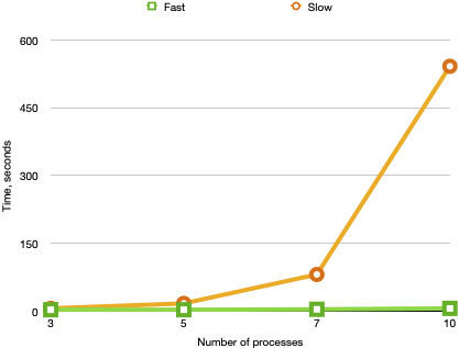
](tutorials/img/counterexample.png)
](tutorials/img/syntaxtree.png)


 or
or